ClarkVision.com
| Home | Galleries | Articles | Reviews | Best Gear | Science | New | About | Contact |
The Exposure Latitude of a Digital Camera
and Comparison to Film
by Roger N. Clark
| Home | Galleries | Articles | Reviews | Best Gear | Science | New | About | Contact |
by Roger N. Clark
Exposure Latitude: The amount of overexposure or underexposure used in acquiring an image (e.g. with a given type of film or a digital camera) that can still produce acceptable results. Exposure latitude is obviously a subjective thing as different people have different ideas at to what is acceptable. You can examine the results in this article and decide what is acceptable for your imaging. The noise in the resulting images was measured and plotted to give quantitative information about the results, and I will present my derivations of exposure latitude based on the noise analysis.
Exposure latitude is related to but different than dynamic range. Exposure latitude depends on dynamic range. The higher the dynamic range, the greater a scene with a lower dynamic range can be recorded with different exposures without compromising highlights and shadow detail. If a large dynamic range scene just matched the capability of the recording medium, then the exposure latitude would be zero. If the scene is low in contrast, the recording system could record the scene at several different exposures and still produce an acceptable image. Thus exposure latitude is also scene dependent.
Methods
In this article I will show some exposure latitude tests from a digital camera and compare those results to print film. The cameras and film used are: Canon 1D Mark II 8-megapixel digital camera, with a Canon 50mm f/1.8 EF II lens operating at ISO 200. The film camera was a Canon Elan II with a Canon 50mm f/1.8 EF II lens (two lenses were used), loaded with Kodak Gold 200 film. The test target used was a Macbeth color chart plus a chart of my own design that has resolution targets in both black and white and color. The test targets have color and black and white patches that cover a 5-stop range in intensities. Exposures were set by metering an 18% reflectance panel. The test targets were set up in full sunlight and exposures obtained around local solar noon on a clear day. The 18% panel was metered with both the digital and film cameras and gave the same answer. The cameras were set to manual and set up side by side on tripods viewing the test target, and a series of exposures were done to cover a large range in light levels: over 23 stops in exposure in full sunlight (-9 to +14 stops). A second series was done with the digital camera only with the target in shade to get to lower levels (to -12.5 stops). Thus, the total range of testing covered -12.5 to +14 stops for a light range of 26.5 stops, or an exposure range of 95 million! The shade results are not quite comparable as light from the blue sky contains very little red light. Thus below -9 stops should be considered as rough lower limit to image quality. During each series, the meter=0 exposure was obtained both at the beginning and end of the test series, and no changes were observed within a fraction of a stop (a test series took about 3 minutes).
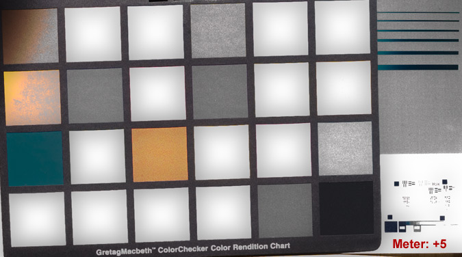
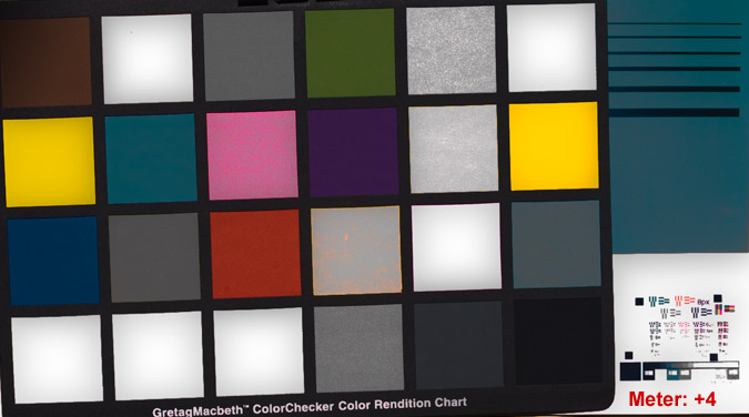
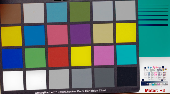
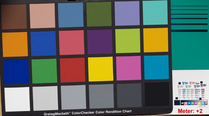
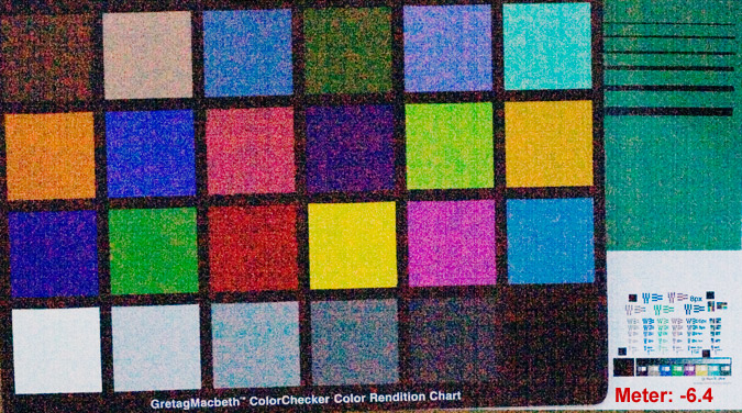
The data below so far shows the 1D Mark II results. The Macbeth color chart, bottom row, forth patch from the left is 20% reflectance, so closest to 18% gray. The brightest patch is +2.2 stops, the darkest -2.7 stops relative to the 20% reflectance patch. The idea is to produce the best image at each exposure.
To produce the best final image at each exposure, I used all methods available to me except I did not do any post raw conversion noise reduction. I found for this series, that I like the results from the Photoshop CS3 beta raw converter best. Thus, all the images from the 1D Mark II were processed in Photoshop CS3 only. Processing included best raw converter setting to produce the best overall image, then using levels and curves in Photoshop to obtain the best image. I used the meter=0 as the reference in my comparisons and tried to make each image a close match to that reference. This included matching the intensity response of the patches as well as color balance. This was done by eye and you will notice small differences between images. For the most part these small differences do not impact the "big picture" conclusions, but with more tweaking one can probably coax out a slightly better image than presented. One important factor at the low end from the digital camera: fixed pattern noise shows as lines (mostly vertical). I also took dark frames and I can subtract out the fixed pattern noise. I will redo the images affected when I have time. That will improve both the visual impression of the image quality and the noise levels.
Digitizing film over such a large dynamic range is also problematic. Both photo lab and my own scans failed at the high end before the film was saturated when done as a negative. To scan the film's high end I scanned the high end as a positive, and that allowed me to capture image information that most people would never see. I visually inspected the negatives to determine if I could see more in the high end than I could scan. It turned out that scanning as a positive, where the density is highest and the scanner output was lowest pushed further into the highlights than I could detect by microscopic examination, and more than could be printed by the photo lab. This means to scan negative film's large dynamic range requires multiple scans in different modes and then merging the scans into one image, no small feat which takes a lot of time. Compare that to the digital's raw image which has all the information in one file and sotware can compress that range into something we can easily see on monitors and prints.
Results
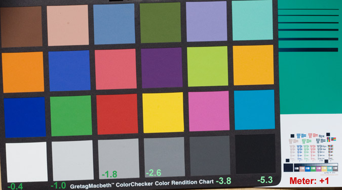
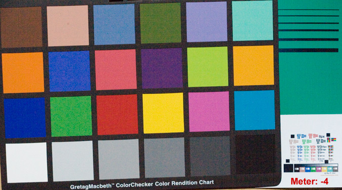
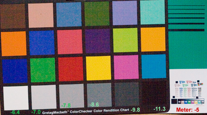
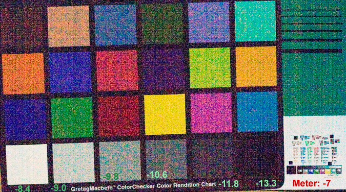
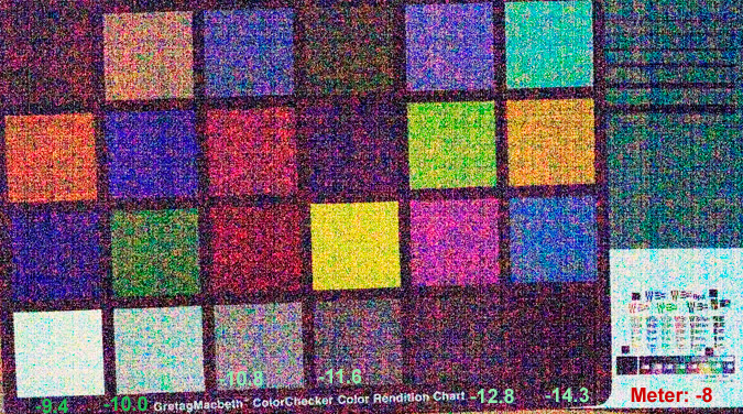
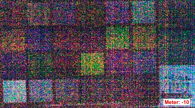
You can look at the images and decide for yourself what is acceptable. Exposures -5 to +2 stops produced excellent images from the digital camera, with no saturation and excellent shadows. The meter +3 second from left white panel is not saturated (59% reflectance) but the whitest panel is, so that is +1.6 stops, so the real dynamic range is +3+1.6 to -5-2.7 = 4.6 + 7.7 = 12.3 stops of excellent image quality with over 7 stops of exposure latitude for this test scene! The meter -7 is still pretty good, for a total range of 14.3 stops! Each can decide on the lower limit to useful images. The meter -8 stops is also pretty good (better than some high speed film images) and there is still information recorded in the -11 stops (label is 11, but actual is 11.4). (Also note the -10 = 10.4 and -11 = 11.4 and were obtained in shadow other in full sun, so light was blue sky and reds are lost. I need to redo the low end).
The noise analysis is shown in Figure 1. Noise was determined using Photoshop CS3 and selecting the a large portion of each gray patch. The R=90% signal-to-noise ratio (S/N) is limited by the target uniformity. The expected S/N would be above 250 if the target were perfectly uniform (photon noise at maximum signal from the 1D Mark II at ISO 200 would give S/N ~ 158 and Bayer conversion averages that to above 250).
A major factor in producing acceptable image quality at the low end is the number of available photons. Table 1 shows the photons incident on the focal plane for light from the 20% reflectance gray patch through a lens transmitting 80% of the light. How many photons actually get detected depends on the transmission through the blur, IR and Bayer filters over the digital camera sensor, the quantum efficiency of the sensor, and the active area of the sensor. The data in Table 1 are interesting because this is a fundamental property of the definition of exposure. For normally metered scene, a 20% diffuse reflectance spot the exposure will deliver about 1300 photons per square micron to the focal plane regardless of f-stop, focal length, or sensor size. You can see that below -7 stops, photon levels are very low. Pixels will collect these photon values times the active area of the pixel. For the 1D Mark II camera used here, multiply these photon levels by about a factor of 50 (the 1D Mark II has 8.2 micron pixel spacing, but not all of the pixel is sensitive to light).
| Exposure (stops) | Photons incident on focal plane through green passband (Photons/sq. micron | Exposure (stops) | Photons incident on focal plane through green passband (Photons/sq. micron | |
| -11.5 | 0.4 | 2.1 | 5,600 | |
| -10.4 | 1.0 | 3.1 | 11,000 | |
| -9.0 | 2.5 | 4.1 | 22,000 | |
| -8.0 | 5 | 5.0 | 42,000 | |
| -7.0 | 10 | 6.0 | 83,000 | |
| -6.4 | 15 | 7.0 | 170,000 | |
| -5.0 | 41 | 8.0 | 330,000 | |
| -4.0 | 81 | 9.0 | 670,000 | |
| -3.0 | 162 | 9.9 | 1,200,000 | |
| -2.0 | 325 | 11.0 | 2,700,000 | |
| -1.0 | 650 | 11.9 | 5,900,000 | |
| 0.0 | 1,300 | 13.0 | 10,000,000 | |
| 1.0 | 2,600 | 13.9 | 20,000,000 |
Another interesting fact is the number of photons the camera detects
on a sunny day. With a sunny-16 rule, the exposure is 1/ISO at f/16
in bright sunlight. That means that at ISO 100, f/16, the exposure
is 1/100 second. Digital cameras detect about 10 to 20% of the light
incident in the focal plane (light is absorbed/reflected from the blur
filter, infrared blocking filter, the color filter, and the sensor quantum
efficiency is about 30 to 40%). Thus with about 1300 photons per square
micron delivered to the focal plane from a 20% reflectance scene, about
150 to 250 get detected in the green passband. This means about 1500
to 2500 photons/second are detected per square micron at f/16 by the
CCD or CMOS sensor with a typical sunlit scene. This is independent
of ISO (ISO on a digital camera is a post sensor amplifier gain; the
sensor has only one sensitivity, given by the Quantum Efficiency). At
f/2 that would be about 100,000 to 160,000 photons detected per second
per square micron in the green passband for a 20% reflectance scene in
full sunlight. Obviously, at f/2, a very short exposure is needed or
the sensor with saturate. The typical capacity of silicon-based sensors
(CCDs and CMOS) is around 1000 to 2000 electrons/square micron. So not
only do larger pixels capture more photons, they store more signal but
both incident light and sensor storage capacities are finite. All this
contributes to dynamic range and exposure latitude. Digital cameras with
larger pixels collect more light because the area of the pixels is larger,
thus they have larger dynamic range and exposure latitude.
Noise Analysis:
Figure 1. Noise analysis as a function of exposure latitude.
The R=90% curve is for data on the lower left white patch;
the R=20% is data from the gray patch on the bottom row,
4th from the left.
The data in Figure 1 shows several effects.
The above two observations are true for both digital and film.
Example Images
The following images are derived from raw conversions of 1D Mark II data. Other images (in-camera jpegs and film scans will be added sometime in the future). ALSO TO BE DONE: fixed pattern dark subtraction which will reduce the fixed pattern noise in the low light images.
On some of the images below, you will see greenish numbers next to or on the bottom row of gray-scale patches. Those numbers are the intensity level in photographic stops below sensor saturation in the green channel. The meter +2 and higher images used Photoshop CS3 "recover" function in the raw converter, which apparently uses lower signals in the red and/or blue channels to recover both intensity information and even color information. At meter +2, only the white patch at the lower left is saturated. At meter +3, some color patches are too bright for color to be recovered but luminance detail was still recovered.
Target in Full Sun


Target in Shade for images below here (blue sky has little red light, so the scene appears different)
| Home | Galleries | Articles | Reviews | Best Gear | Science | New | About | Contact |
http://clarkvision.com/articles/exposure_latitude-1
First published April, 2007.
Last updated November 16, 2008