ClarkVision.com
| Home | Galleries | Articles | Reviews | Best Gear | Science | New | About | Contact |
Digital Camera Reviews and Sensor Performance Summary
by Roger N. Clark
| Home | Galleries | Articles | Reviews | Best Gear | Science | New | About | Contact |
by Roger N. Clark
Data on this page are from the references below and from the Digital Camera Sensor Analysis pages on this site: http://clarkvision.com/reviews/
Modern digital cameras contain electronic sensors that have predictable properties. Foremost among those properties is their relatively high Quantum Efficiency, or ability to absorb photons and generate electrons. Second is that the electronics are so good in most cameras, that noise is under 2 electrons and rarely worse than about 15 electrons from the sensor read amplifier. With the low noise and high Quantum Efficiency, along with the general properties of how the sensors collect the electrons generated from photons, it is possible to make general predictions about camera performance. An important concept emerges from these predictions that we are reaching fundamental physical limits concerning dynamic range and noise performance of sensors. But downstream electronics after the signal is read from the sensor is still a limiting factor. See References 18, 20 (from electronic sensor companies) and Reference 24 (from University class lecture notes) for more details about the above well-established concepts and how electronic sensors operate.
The ideal sensor absorbs every photon, each photon would liberate an electron and every electron would be collected and counted to form the image, all done with no added noise. Would images from such a camera be perfect (no noise and infinite dynamic range)? NO! All measurements of light (photons) still have inherent noise, called photon noise. The dynamic range is not infinite, but would have a maximum of the number of photons collected. For example, if you collected 1,000 photons, the dynamic range would be 1000:1 or almost 10 photographic stops.
Dynamic range per pixel is defined in this document and elsewhere on this site as:
Traditionally, the minimum discernible signal has been limited by the sensor read noise and downstream electronics. But circa 2016, read noise is near 1 electron in some consumer cameras, and sub-electron sensors are operational in labs and will likely reach consumer cameras soon. That means single photons can be detected. Such photon counting systems require a more detailed equation than equation intro-1.
The traditional definition:
In the new circa 2016+ era of low noise sensors, the equation is:
In the perfect sensor (above), the read noise would be zero, but the minimum discernible signal is 1 photon and the noise would be square root 1 = 1 photon, giving the dynamic range of 1000 (in the 1000 photon example above). In real digital cameras, amplifier and analog-to-digital converter noise contributes to the apparent read noise, so each ISO has a different measured read noise, resulting in changes in the dynamic range with different ISOs. Thus, in most digital cameras, dynamic range in the image data for a pixel is less than the dynamic range of a pixel at the sensor due to downstream electronics limitations, especially at low ISO. The equation intro-3 above is used for the measured dynamic range per pixel out of the camera. This article will present data and models of the read noise, full well capacity, dynamic range and other parameters. (Note Oct 2016: the above equations are to clarify the changing landscape of sensors; the data below on dynamic range still uses equation intro-2a. When this article get a coming major update, I will update the dynamic range numbers to equation intro-3. Most numbers will not change and none will change significantly.)
The dynamic range chosen for clarkvision uses the common standard of signal-to-noise ratio, S/N = 1.0. Some other sites use other values, e.g. 4. Note in an image context image info can be seen well below S/N = 1. Fine grained film on the same image scale has S/N less than about 20, so so in my opinion, setting a noise floor above S/N = 1 is inconsistent with observed image quality.
In the physics of photon counting, the noise in the signal is equal to the square root of the number of photons counted because photon arrival times are random. The reason for this dependence is Poisson Statistics (Wikipedia has an excellent article on Poisson statistics). For example Table 1 shows the signal-to-noise ratio when detecting different numbers of photons.
| Photons | Noise | Signal-to-noise Ratio |
| 9 | 3 | 3 |
| 100 | 10 | 10 |
| 900 | 30 | 30 |
| 10000 | 100 | 100 |
| 40000 | 200 | 200 |
| 90000 | 300 | 300 |
Why is this important? It turns out that the noise making up the majority of images we view from good modern digital cameras is dominated by photon counting statistics, not other sources. So to make an image with a high signal-to-noise ratio, one must collect the most photons possible. Modern electronic sensors have a method for collecting the electrons from photons (they are called photoelectrons) and storing them in the sensor until the electrons are transferred from the chip to the electronics in the camera where the signal is amplified, digitized and converted into an array of numbers to be recorded in a memory card and later displayed as an image by a computer.
Another reason photon noise is important is that in a photon noise limited system, a single measurement (e.g. the signal in a single pixel), one knows the signal, the noise and the S/N. There is no need to make multiple measurements or do statistics on many pixels.
Both CCD and CMOS silicon sensors used in today's digital cameras exploit a property of semiconductors. Silicon is a semiconductor. When a photon is incident on the silicon, the photon may be absorbed, and the energy from the photon excites an electron, moving it into what is called the "conduction band" from the low energy state called the "valence band." There is an energy gap, called the "band gap" across which the electron must move. The band gap sets the lower limit (longest wavelength) of the photon energy that can be absorbed by the electron to move it into the conduction band (see Reference 24 for more details). For silicon, that wavelength is about 11,000 angstroms (1.1 microns) in the infrared. Photons with wavelengths shorter than this value have higher energies, and those energies include wavelengths visible to our eyes, called the visible spectrum. Once an electron is excited into the conduction band, the challenge is to capture it before it moves far (like electrons flowing great distances in a copper wire, where electrons are flowing in the conduction band).
The electric field in the silicon is modified by adding impurities (called doping, e.g. parts per million of arsenic or boron or other elements in the columns in the periodic table on each side of silicon) to control were the electrons flow. Voltages are applied to the silicon, and when a photon is absorbed, primarily by the electrons in the valence band, the electrons will be excited into the conduction band and flow toward positive voltage. These electrons are also called "photoelectrons." The local electric fields produced by the doping and applied voltages trap the electrons in small regions (pixels in imaging sensors). The trapped electrons correspond to absorbed photons, and in the sensor industry, photons and electrons (photoelectrons) are interchanged in describing sensor performance.
Thus, when a digital camera reads 10,000 electrons, it corresponds to absorbing 10,000 photons. So the graphs shown in this article that are in units of electrons, like Sensor Full Capacity, also indicate how many photons the sensor pixel captured. The camera electronics also generates a small amount of noise, and from a measurement perspective, that noise is in electrons and the noise source, whether camera electronics or from photon noise, gets mixed into the images you observe. With measurement techniques, the various noise sources can be isolated and their individual contributions measured. This article summarizes available data for numerous sensors, both digital cameras and from sensor manufacturer data sheets.
Fundamental factors set sensor performance of semiconductors like CMOS and CCDs. These include the absorption length in silicon, the efficiency of photon absorption (which is very high, typically 40-50% for modern digital cameras), and electron charge density in the silicon. Blue wavelength photons have shorter absorption lengths in silicon than red or green photons. Major factors in limiting the maximum number of electrons captured in a semiconductor image sensor are the absorption length and electron densities. The wavelength-variable absorption lengths in silicon are exploited in the development of the Foveon sensor and some Sigma digital cameras, for example, allowing a single spatial pixel to separate red green and blue colors. Unfortunately, the absorption lengths overlap too much for fine wavelength discrimination. Table 1b shows the absorption lengths.
| Wavelength (angstroms) | Wavelength (microns) | Color | Absorption (1/e) Length in Silicon (microns) |
| 4000 | 0.40 | ~violet | 0.19 |
| 4500 | 0.45 | ~blue | 1.0 |
| 5000 | 0.50 | ~blue-green | 2.3 |
| 5500 | 0.55 | ~green-yellow | 3.3 |
| 6000 | 0.60 | ~orange | 5.0 |
| 6500 | 0.65 | ~red | 7.6 |
| 7000 | 0.70 | ~red limit | 8.5 |
The absorption lengths of photons in Table 1B are the 1/e depth (e = 2.7183), or the 63% probability of a photon being absorbed along that length. Some photons can, in reality travel several times this distance before being absorbed. These absorption lengths impact performance as pixels become smaller. For example, small sensor digital cameras currently have pixels smaller than 2-microns. What happens when red photons enter the silicon and after 5 microns only 63% of them are absorbed, and after 10 microns (10 pixels) 13% are still moving through the silicon being absorbed at greater distances from the original pixel? Well, it can't be good in terms of a color imaging sensor. If the absorbed photon results in an electron in the conduction band, it likely contributes to photons several pixels away from the target pixel.
Different Photography Situations
The sensor data in this article can be applied in multiple ways. Early in the Digital Camera era, the number of pixels was relatively similar and sensor sizes varied. But now (2009 and beyond) there is a large variety of megapixels to choose from within one sensor size, and the choices will likely be greater in the future. Some discussions on the internet have debated pixel size where some take extreme positions of larger pixels are better and others claiming smaller pixels are better. In practice, there are situations where large and other situations where smaller pixels will produce better images. But there are also situations where it matters so little, only a lab measurement could tell the difference! In theory, if the read noise were zero, one could synthesize in post processing, any equivalent pixel size. Some cameras are getting close to this ideal. Sensor data will be presented which will help resolve such differences.
However, I want to be clear regarding the sensor data: the pixel and its size is only a holder for the photoelectrons. It is the lens that delivers the photons to the sensor. Just because a pixel is larger does not mean that it will produce better or lower noise images if the lens and exposure time does not fill the pixel with enough light (and thus, photoelectrons). If one is working above base ISO, the pixel will not be filled to its full capacity. The larger pixel has the potential to collect more light. But larger pixels see larger angular areas from the lens, so resolve less detail. There is a trade between the lens collecting the light, the focal length spreading out the light, the pixels chopping up the light. and the exposure time limiting the light collected. For the impact on an image of these parameters, the full system must be considered. That is done in the article: Telephoto Reach, Part 2: Telephoto + Camera System Performance (A Omega Product, or Etendue) (Advanced Concepts). This article simply describes the capabilities of sensors, the pixels in those sensors and their potential to deliver quality images.
Extreme pixel sizes generally do not produce high quality images. For example, if large pixels are better, consider a camera with the pixel so large, there is only one pixel. Obviously, there is little image information and the image would not look good. On the internet, people argue about smaller pixels, and say, after all film has grain (single pixels) with only 1 bit of dynamic range per grain (on or off). But film grain has a 3-dimensional structure and it is grain clumps which provide tonality, not individual grains. The 3-dimensional grain distribution also gives film its characteristic curve so that once a grain has absorbed a photon it is no longer sensitive, and within a grain clump it is the probability of another grain absorbing a photon that gives a logarithmic response of the grain clump, extending its dynamic range. These are properties unlike the 2-dimensional grid In a digital camera electronic sensor. As pixels become smaller, signal level drops per pixel and read noise may become more dominant, and that limits small pixel performance. Yet more pixels provide more resolution (if the lens can deliver that resolution), so clearly there are optimums in image quality from a single large pixel to small pixels dominated by noise. But different situations call for different sized pixels, so there is not one optimum.
There are generally 4 imaging situations where pixel and sensor performance will influence the quality of the resulting images. We will make the assumption that output is a "print," but it could also be a monitor or some other output device.
1) Full sensor, maximum print size. Focal length is changed to frame the scene and no cropping is done. More pixels shows finer detail, but if sensor size is not increased, the pixels get noisier as the sensor is divided into smaller and smaller pixels. More pixels deliver finer but noisier details. A larger sensor and greater focal length can maintain low noise and deliver finer details assuming the lens scales with the sensor (e.g. use the same f/ratio and exposure time). The apparent image quality is given by the Full sensor Apparent Image Quality, or FSAIQ metric.
2) Full sensor, constant print size. No cropping. If your image has more pixels, you will get more pixels per inch on the print. As the number of pixels increases for constant sensor size, the light received per unit area stays relatively constant until pixels become very small, then light levels, dynamic range drops and read noise per unit area increases. For constant print size, as long as there are enough pixels (e.g. enough pixels per inch to be limited by the printer), increasing the number of pixels will not improve, nor harm print quality, but as pixels become very small, read noise and dynamic range will drop, hurting the output. The FSAIQ metric is best metric for this situation but once the pixel density matches or exceeds the output device, no further improvement is likely and when pixels become very small, image quality will drop assuming the detail can be resolved with the human eye.
3) Focal Length Limited, image is cropped but constant print size. For example, you want to print your cropped subject on 8x10 paper. Thus, if you have more pixels, the print will have more pixels per inch. For constant sensor size, more pixels provide for more fine detail. As the number of pixels increases for constant sensor size, the light received per unit area stays relatively constant until pixels become very small, then light levels and dynamic range per unit area drops and read noise per unit area increases. An example might be you want to make and 8x10 print of the Moon. A 1 megapixel camera with large pixels will give high dynamic range and low noise, but not much detail. Decreasing the pixel size with the same focal length lens (assuming the lens can deliver more detail) will provide more resolution on the print and that can be more important than higher dynamic range and lower noise. The FLL-AIQ1600 metric is the best metric for this situation.
4) Focal length limited, image is cropped but printed at maximum size. If you have more pixels, for example, you can print larger. For example, you want the largest print possible of a distant bird. Smaller pixels will provide more resolution on the bird, but with a constant sensor size, each pixel will collect less light and have lower signal-to-noise ratios. As long as noise does not become too noticeable, and dynamic range is not a limiting factor, the improved resolution will be seen by most viewers as more important. Maximum megapixels for a given sized sensor is probably the best metric, as long as the lens can deliver the image detail and noise and dynamic range are not compromised too severely. Maximum megapixels also means the smallest pixels, so a metric is 1/pixel pitch. Note, diffraction is the ultimate limit to image detail.
Complications regarding the perceived performance of pixels, pixel size and sensor size in digital cameras over the last decade (about 2000 to 2009) is a significant refinement in technology. While the quantum efficiency of sensors in digital cameras has not really changed much, other factors that have improved include: fill factor (the fraction of a pixel that is sensitive to light), higher transmission of the filters over the sensor, better micro lenses, lower read noise, and lower fixed pattern noise.
Current DSLRs (2010 - 2014) with similar sensor sizes have a range of about two in pixel size. Whether image detail at the cost of noise and possibly dynamic range is more important to you depends on your tastes and on your application. There is no perfect sensor, and large or small pixels in a given sensor size will give better performance in different situations. The sensor data on this page will help you to understand what these trades are, how technology is changing, and should enable you to make better decisions for your imaging needs.
Image quality is subjective and the bottom line is lighting, composition and subject are more important than the inherent image quality that a camera delivers. I have been studying sensor performance for two reasons: intellectual curiosity and a better camera for astrophotography. In comparing results on this page, do not get too carried away with over-interpreting the results. You would probably do better spending your time out photographing and refining your knowledge on lighting, composition, and subject. (see: http://clarkvision.com/articles/lighting.composition.subject).
What follows are sensor performance data. For each property, note the trends. See the section on the Sensor Performance Model. for details of the models.
A growing misinterpretation of results like those I present below is that larger pixels are less noisy. The signal-to-noise ratio is dependent on the amount of light collected, and the light collected is delivered by the the lens. It is the lens, it's focal length and the exposure time that determines the amount of light collected. A larger pixel only enables more light to be collected, but at the expense of less detail resolved (given the same focal length lens).
But consider a big bucket and a
little bucket. Turn on some water for a short time in each bucket.
Which bucket has more water? Both buckets contain the same amount of water.
It is the force and duration of water that determines how much water
is in the bucket, not the size of the bucket. The larger bucket only allows
more total water to be poured into the bucket. Same with pixels.
So in the sensor analyses below, the size of the pixel only enables more light
(electrons) to be stored in the pixel. It is up to the lens and
exposure time to actually deliver those photons. For more on this
subject, see:
Camera System Performance (A Omega Product, or Etendue)
The property that describes the capacity to hold the electrons in each pixel that are generated from photons is called the "Full Well Capacity." As a pixel holds more electrons, the charge density increases. There are finite upper limits to the charge density of electron storage, and undesirable side effects can occur, including charge leaking into adjacent pixels, called blooming (e.g. see reference 19). Blooming was common in early CCDs causing streaks from bright objects in the image.
Full well capacities of some cameras and sensors are shown in Figure 1. Because of the finite and fixed absorption lengths of photons in silicon (Table 1b), the full well capacities are basically a function of pixel area (and not volume).
The bottom line for the full well capacity from the recent trends in the Canon line, is
that sensor technology in that line is mature and the choice scales with pixel size.
But note, this is just one of several parameters.
Full well capacity is important for maximum signal-to-noise ratio and dynamic range. Figure 2 shows the signal-to-noise ratio at ISO 100 on an 18% gray card. Eighteen percent is close to the average scene intensity in regular photographs, so Figure 2 shows the typical signal-to-noise ratio in a typical photograph. Dynamic range is shown in Figure 4, and shows a small trend with pixel size. Because this trend scales directly from the square root of the full well capacity and we see the same maturing of technology with recent Canon cameras as we do in Figure 1.
Full well capacity does not necessarily indicate low light performance even though more electrons (electrons excited and collected by the absorption of photons) means better low light performance. For example, the Nikon D50 plots low in Figure 1. But that full well occurs at ISO 200 where most other cameras are at ISO 50 to 100. Thus, the Nikon D50 is actually more sensitive, and this is indicated on the Unity Gain ISO data discussed below and presented in Figure 6 (where the Nikon D50 plots very high). Low light performance with a given lens is controlled by the Quantum Efficiency of the device combined with the total photons the device collects.
For detecting the lowest signals, read noise is a controlling factor. Read noise is expressed in electrons, and represents a noise floor for low signal detection. For example, if read noise was 10 electrons, and you had only one photon converted in a pixel during an exposure, the signal would mostly be lost in the read noise. (It is possible to see an image where the signal is 1/10 the read noise, where one uses many pixels; see: Night and Low Light Photography with Digital Cameras http://clarkvision.com/articles/night.and.low.light.photography.) Older CCDs tend to have read noise levels in the 15 to 20 or more electrons. Newer CCDs in better cameras tend to run in the 6 to 8 electron range, and some are as low as 3 to 4 electrons. The best CMOS sensors currently have read noise less than 2 electrons and the Canon 1DX shows less than 1 electron at very high ISOs. Figure 3 shows read noise for various cameras and commercially available sensors. One can see that there is no real trend with pixel pitch.
Read noise dominates the signal-to-noise ratio of the lowest signals for short exposures of less than a few seconds to a minute or so. For longer exposures, thermal noise usually becomes a factor. Thermal noise increases with temperature, as well as exposure time. Thermal noise results from noise in dark current, and the noise value is the square root of the number of dark-current generated electrons. Thermal noise is discussed in more detail below.
A large dynamic range is important in photography for many situations. The pixel size in digital cameras also affects dynamic range. Sensor dynamic range is defined here to be the maximum signal divided by the noise floor in a pixel at each ISO. The noise floor is a combination of the sensor read noise, analog-to-digital conversion limitations, and amplifier noise. These three parameters can not be separated when evaluating digital cameras, and is generally called the read noise. As you might have surmised by now, with the larger pixels potentially collecting more photons, those larger pixels can also have a higher dynamic range. Figure 4 shows the maximum dynamic range possible per pixel from each sensor, based on full-well capacity / best read noise, assuming no limitation from A/D converters. Figure 5 shows the measured dynamic range from 3 cameras with significantly different pixel sizes as a function of ISO. The full sensor analyses for these 3 cameras (as well as other cameras) can be found at: http://clarkvision.com/articles/index.html#sensor_analysis. One sees that actual dynamic range of a digital camera decreases with increasing ISO as long as the range is not limited by the A/D converter. At higher ISOs, it is obvious that large pixel cameras have significantly better dynamic range than small pixel cameras, but at low ISO there is not much difference. If 16-bit or higher analog-to-digital converters were used, with correspondingly lower noise amplifiers, the dynamic range could increase by about 2 stops on the larger pixel cameras. The smallest pixel cameras do not collect enough photons to benefit from higher bit converters concerning dynamic range per pixel.
NOTE: Unity Gain is a flawed concept in my opinion. It is included here for historical reference. Contrary to some posts on the net, I did not start this concept. It seems like a good idea: that the fundamental counting unit is one quanta: an electron. It seemed that one should not need to digitize a signal finer than 1 electron. In the early days of digital cameras (before about circa 2008), the electronics in digital cameras were too noisy to counter the theory. But since then digital cameras have substantially lower noise. Read noise at high ISOs are commonly less than 2 electrons. But this is only obtained when ISOs are much higher than Unity Gain. Clearly there are advantages to ISOs beyond Unity Gain. The fundamental reason Unity Gain is not relevant is because the sensor in a digital camera is an analog system, not digital. The signals from the sensor are analog and only after amplification is the signal digitized.
The following is for historical reference.
A concept important to the fundamental sensitivity of a sensor is the Quantum Efficiency. But in terms of camera performance other factors also play a role, including the size of a pixel, and the transmission of the filters over the sensor (the Bayer RGBG filter, the IR blocking filter, and the blur filter). Larger pixels enable the collection of more light, just like a large bucket collects more rain drops in a rain storm. But the large pixel comes at a cost: less resolution on the subject (less pixels on the subject).
A parameter that combines the quantum efficiency and the total converted photons in a pixel, which factors in the size of the pixel and the transmission of the filters (the Bayer RGBG filter, blur filter, IR blocking filter), is called the "Unity Gain ISO." The Unity Gain ISO is the ISO of the camera where the A/D converter digitizes 1 electron to 1 data number (DN) in the digital image. Further, to scale all cameras to equivalent Unity Gain ISO, a 12-bit converter is assumed. Since 1 electron (1 converted photon) is the smallest quantum that makes sense to digitize, in theory there is little point in increasing ISO above the Unity Gain ISO (small gains may be realized due to quantization effects, but as ISO is increased, dynamic range decreases). EXCEPT THE THEORY IS FLAWED. There is a caveat to this idea: fixed pattern noise may still be a factor and in some cameras, a higher ISO than unity gain is needed to reduce the apparent fixed pattern noise. Figure 6 shows the Unity Gain ISO for various cameras and sensors that can be purchased from manufacturers. It is clear that there is a trend in ISO performance as a function of pixel size. Gains for various cameras are shown in Table 3 as a function of ISO. Note in practice for 14-bit systems lower ISO may be employed if the A/D converter does not limit performance. In comparing actual performance of 14-bit A/D converters (e.g. see Figure 8a) and the read noise in Table 4, the lowest apparent read noise performance remains similar (~ISO 1600) for both 12-bit DSLRs and 14-bit DSLRs. But many cameras have pattern noise at low ISO, including ISOs above Unity Gain. Optimum low light performance is at ISOs at or above Unity gain and high enough where pattern noise is no longer apparent. In many DSLRs, this is around ISO 1600 (see individual camera sensor analyses). In practice, set the gain at the nearest 2x ISO (e.g. ISO 400, 800, 1600, 3200), as the data obtained at other ISOs may be simply multiplied by the camera's digital processor in some cameras. In many cases, it is usually difficult to see the performance difference between ISO 800 and 1600 except for the lower dynamic range decrease at the higher ISO, or the higher fixed pattern noise at lower ISOs.
One can find on the internet discussions about the "Native ISO" for a camera.
There is really no such thing. ISO is simply a post sensor gain followed by
digitization. ISO settings are needed mainly to compensate for
inadequate dynamic range of down stream electronics. One could
specify ISO such that downstream electronics digitize the full range
of signal up to the full well capacity. Some may say that
is the native ISO, but there is no inherent advantage to this ISO, and in
many applications is less than ideal. Digitizing the full range,
assuming one fills that range with electrons from optimum
exposure, maximizes signal-to-noise ratio at high signals
(this is the concept of use the lowest ISO on the camera, and
"expose to the right." However, this range provides poor
digitization of the low end of the signal, and depending on the
camera can have side effects like pattern noise. Alternatively,
working at higher ISOs digitizes the low end of the signal range
better with the sacrifice of losing the high end of the range.
See
"What is ISO on a digital camera?
ISO Myths and Digital Cameras" for more information on ISO.
Unity Gain ISO describes the high signal part of an image (the highlights) at high ISO, and apparent read noise the performance corresponding to the low signal end of the photograph. But if a camera was delivering more photons to a pixel, then read noise alone does not give a complete story of the performance in the shadows. The "Low-Light Sensitivity Factor" describes the high iso shadow performance per pixel (Figure 7). It also describes the low light performance in shadows of exposures up to tens of seconds at high ISO.
In astrophotography, a high Low-Light Sensitivity Factor would record the most faint stars, at least for exposures where thermal noise did not dominate. However, this low light sensitivity factor does not apply to stars. And if not stars, then not other subjects. For example, stars in the focal plane are small disks, spread by diffraction, atmospheric turbulence, and lens aberrations. Thus, spread over several pixels, and more pixels in a camera with smaller pixels. For SUBJECT sensitivity a better metric may be signal density divided by read noise density (see Figure 10). This section will be changed after more testing. Note the 7D in Figure 7 shows a much lower factor than the 1D Mark IV, yet the 7D records stars at least as faint as the 1DIV, and perhaps slightly fainter. See Nightscape Photography with Digital Cameras for example images that prove this. A contributing factor in low light long exposure factor is also the detrimental effects of noise from dark current. That too will be factored into a new measure.
At high signal levels (most of the range of a digital camera image), noise per pixel is dominated by photon noise, the inherent random arrival times of photons at the sensor. At the lowest signal levels, other sources contribute. There is sometimes confusion over what are the sources of such low level noise. For example, Table 4 below shows apparent read noise is high (when expressed in electrons) at low ISO and decreases with increasing ISO. Figures 8a and 8b show the sources and reasons for these trends. At low ISO large pixel cameras, typical of DSLRs collect enough photons that photon noise is small compared to read noise and noise from the analog-to-digital converter (ADC). Some call this quantization noise, and while such noise contributes to the total ADC noise, other noise sources in the ADC stage dominate, especially on newer cameras with 14-bit ADCs (the Canon 40D in Figure 8a). On small pixel cameras, the analog gain is high enough that at low signals, read noise dominates the noise sources and ADC noise is a small factor (Figure 8b). The small pixel camera in Figure 8b looks like is has better low ISO performance than the large pixel cameras in Figure 8a, but that is not the case, because the large pixel cameras collect many times more photons/pixel in a given exposure.
Thermal Noise from Dark Current
On long exposures, electrons collect in the sensor due to thermal processes. This is called the thermal dark current. As with photon noise, the noise from thermal dark current is the square root of the signal. One can subtract the dark current level, but not the noise from the dark current. Many modern digital cameras have on sensor dark current suppression, but this does not suppress the noise from the dark current. It does, however, prevent uneven zero levels that plagues cameras before the innovation (Canon cameras before circa 2008). Examples of this problem are seen at: Long-Exposure Comparisons.
Noise in an image is:
N = (S + r2 + t2)1/2 = (S + r2 + dc * e)1/2, (eqn 1a)
S = P * e, (eqn 1b)
Signal-to-Noise Ratio, SNR = S / N, (eqn 1c)
where N = total noise in electrons, S = number of photons (signal), r = apparent read noise in electrons (sensor read noise + downstream electronics noise), and t = thermal noise in electrons. The thermal noise equals the square root of the dark current per second, dc, times the exposure time in seconds, e. The signal, S, is proportional to the photon arrival rate, P, times the exposure time, e. Noise from a stream of photons, the light we all see and image with our cameras, is the square root of the number of photons, so that is why the S in equation 1 is not squared (sqrt(S)2 = S). Both the total photons counted, S, and the thermal noise, t, are functions of exposure time. S is directly proportional to exposure time. Thermal noise is is related to dark current. Dark current is usually expressed as electrons/second, and the noise is the square root of the electrons, so thermal noise is proportional to the square root of the exposure time.
See individual sensor evaluations for details on dark current for a given camera.
Diffraction also limits the detail and contrast in an image. It is the loss of contrast and detail that limits the Apparent Image Quality (below). As the pixel size becomes smaller, lenses must be used at lower f/ratios and those lenses must deliver better performance in order to increase Apparent Image Quality. Few lenses are diffraction limited at f/8 over their entire field of view, so this is an optimistic upper limit to image quality.
Pixel Density
In situations where the output image size is limited, like constant
print size, the effects of the total of pixels in a unit area
has a more important effect on image quality than single pixels.
This section shows the signal per unit area (Figure 10),
read noise per unit area (Figure 11) and dynamic range
per unit area (Figure 12). In presenting data per unit area,
the advancements in technology become more apparent. If technology were
constant and pixel size varied, the solid lines in Figures 10 -13
indicates the trends. But in general we see that older cameras
plot worse than the model lines while newer cameras plot on or better
than the models.
Full Sensor Apparent Image Quality (FSAIQ)
Apparent image quality is a subjective measure, that includes resolution and signal-to-noise ratio. While this is not a new concept, I present my own working definitions.
Image quality depends on the imaging situation. As described in the beginning sections of this article, if you want maximum image quality and can choose the focal length to make use of the entire sensor (e.g. landscape photography), the image quality metric will be different than if you want maximum detail on a subject, like a bird, that is small in the frame and you can not increase focal length. The first situation regards use of the full sensor, so "Full Sensor Apparent Image Quality" is important, FSAIQ:
FSAIQ = StoN18 * MPix / 20.0 = sqrt(0.18*Full well electrons) * Mpix / 20.0,
where StoN18 is the signal-to-noise delivered by the sensor on an 18% gray target, assuming a 100% reflective target just saturates the sensor, and Mpix is the number of megapixels. StoN18 is computed from pixel performance before Bayer de-mosaicing: indicative of the true performance of each pixel. Table 2 shows calculated FSAIQ. Actual image quality depends on the lens delivering a certain resolution, so use these values as a rough guide of what might be possible. More information on FSAIQ and comparison to film can be found at: http://clarkvision.com/articles/film.vs.digital.summary1.html.
The data for FSAIQ for some sensors in Figure 13 plot below the model curves. This is best seen in the trend below the 1.6x-crop model. Those points represent older cameras that had lower efficiency (e.g. the Canon 10D, plotting at 7.4 micron pixel pitch), probably due to lower fill factors, lower quality microlenses, and lower quantum efficiencies. The newer cameras plot close to the model lines. The Nikon D3 plots below the model because of the reported low full-well capacity (more data at ISO 100 are needed to confirm the D3 full-well capacity). The Canon 7D and 1D Mark IV have higher system sensitivities than the model so are plotting a little above the models.
Note the Canon 7D in Figure 13 falls above the red dashed line. The red dashed lines is decreasing due to loss of detail and contrast from diffraction at f/8. Thus, a lens working faster than f/8 and delivering the detail better than an f/8 diffraction limited lens is needed to enable the 7D sensor to give the indicated quality in its images. That requires a very high quality lens.
The FSAIQ model and sensor data in Figure 13 is for the lowest ISO filling the
pixel with electrons. FSAIQ for higher ISOs drops approximately with the
square root of the ISO, so quadruple the ISO and the FSAIQ drops by 2x.
If new sensors came out with higher quantum efficiency (about a 2x improvement
is possible), the FSAIQ would be increases by the square root of the
increase, so a 1.4x improvement is possible.
Focal Length Limited Apparent Image Quality FLL-AIQ
Now we look at image quality in situations where you want to resolve the most detail as possible on a subject, for example, the Moon with a sort telephoto lens, or a bird or other subject when it is small in the frame.
We first consider such a focal length limited situation where one wants to make the same sized output, e.g. a print. For example, you want to make an 8x10 inch print of the Moon. To get maximum detail on the Moon, one needs the smallest pixels for a given focal length as long as the lens can deliver the detail, and such that the pixels are not too small that the small pixel result in too much apparent noise (low signal-to-noise ratios) and that dynamic range is not impacted. The focal length limited constant output apparent image quality, at ISO 1600, FLL-AIQ1600, is:
FLL-AIQ1600 = pixels/mm * StoN18 at ISO 1600 * square root(dynamic range density/15 stops)/42
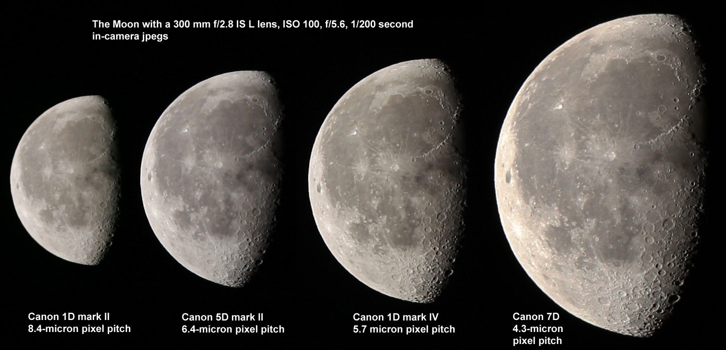
Focal Length Limited Apparent Image Quality FLL-AIQ-MAX
In focal length limited situations where you want the maximum detail on a subject, the highest resolution will be delivered by the sensor with the smallest pixels, assuming the lens can deliver the detail. Most will judge the highest image quality on the image with more fine detail even with more noise, as long as the noise is not excessive and the dynamic range is adequate. The best metric for this situation is the inverse of the pixel size, as given in the Camera Sensor Figure of Merit (CSFM) section below.
An illustration of the inverse pixel size is illustrated in Figure 15. The moon was photographed with the same lens on four cameras, ranging from 8.2 micron pixels to 4.3 micron pixels. The image with 4.3 micron pixels shows more detail. Note, there is no crop factor multiplier effect. See Crop Factor for more details.
Camera Sensor Figures of Merit (CSFM)
The AIQ function above requires reliable sensor performance data which does not exist for many sensors. Also, when new cameras are introduced, one might want some simple prediction of sensor performance based on data that the consumer might readily obtain. So I have come up with a simple equation:
Camera Full Sensor Figure of Merit (CFSFM) = megapixels * pixel pitch.
Pixel pitch is proportional to the square root of the pixel density, and pixel pitch is also related to signal-to-noise ratio, which is a main property of my AIQ function. But the above equation does ignore quantum efficiency, filter transmission and fill factor variations which is better represented in the S/N in AIQ model above. However, we do not have raw data and S/N sensor info for many cameras, so figures of merit may be good overall indicators. I'll add computed figures of merit as time permits, but you can easily use the data in the Table 2 to compute the figures or merit for various cameras. However, the figures of merit does ignore the small pixel effects of vanishing dynamic range as pixel size decreases, and lower image detail due to diffraction effects, which is in the AIQ models.
Example Camera Sensor Figures of Merit values:
CFSFM = Camera Full Sensor Figure of Merit
FLLCSFM = Focal Length Limited Camera Sensor Figure of Merit
IMPORTANT NOTE ON INTERPRETING FLLCSFM. This is the focal length
limited case and only applies to true focal lengths. For example,
the FZ50 has an attached 35-420 mm equivalent lens, but the true
focal length is only 7.4 to 88.8 mm. If you took a picture of the Moon
at 88.8 mm (max zoom) on the FZ50 and compared it to an image taken with
an 88.8 mm lens on a Nikon D3, the FZ50 image would show more detail.
But if you had a longer focal length about 3 times longer on the D3, the
two cameras would produce similar spatial detail (but the D3 would be higher
signal-to-noise), and with longer focal lengths, the D3 would show more detail.
So ratios of the FLLCSFM will indicate the ratios in true focal lengths
needed to show similar detail on a small subject in the images from each
camera. For example, with the Canon 7D, a 180 mm lens would produce
similar detail on the subject as the FZ50 at maximum zoom, but again the
7D would have higher signal-to-noise images. The CFSFM indicates which camera
has higher quality pixels, and FLLCSFM indicates the relative resolution
for the same true focal length lenses. It is physically impossible for
both metrics to be the maximum for the same camera.
Camera              Megapixels  Pixel Pitch  CFSFM         FLLCSFM
                       (MP)      (microns)  (MP*microns)  (200/pixel pitch in microns)
Pentax 645D           40.4         6.0       242             33   (Kodak KAF 40000 sensor)
Nikon D800            36.3         4.88      177             41
Sony A900, Nikon D3x  24.4         5.95      145             34
Canon 1Ds Mark III    21.1         6.4       135             31
Canon 5DIII           22.3         6.25      139             32
Canon 5D Mark II      21.1         6.4       135             31
Nikon D4              16.2         7.3       118             27
Nikon D3              12.1         8.46      102             34
Canon 1D Mark IV      16.1         5.7        95             35
Nikon D7000           16.2         4.8        78             42
Canon 7D              17.9         4.3        77             47
Canon 1D Mark III     10.1         7.2        73             28
Canon 50D             15.0         4.7        71             43
Nikon D90             12.3         5.5        68             36
Canon 1D Mark II       8.2         8.2        67             24
Canon 40D             10.1         5.7        57             35
Canon 30D              8.2         6.4        52             31
Olympus E3            10.0         4.7        47             43
Olympus E300           8.0         5.3        42             38
Sigma DP1              4.7         7.8        37             26
Sigma SD10             3.5         9.0        31             22
Canon G10             14.7         1.72       25            116
Sony W300             13.4         1.8        24            111
Fuji HS30 EXR         16.0         1.389      22            144
Panasonic FZ50        10.0         1.97       19.7          102
Fuji F30               6.3         2.67       16.8           75
Canon S70              7.1         2.3        16.3           87
Panasonic FZ18         8.1         1.76       14.3          114
Sony H5                7.2         1.87       13.5          107
Canon S3               6.0         2.0        12.0          100
The sensor models in this article are simple but they accurately describe many sensors. Note the greater the distance in data points from the model generally occurs for older sensors. e.g. probably due to lower fill factors, lower quality microlenses, and lower quantum efficiencies. Newer sensors tend to plot closer to the model.
Two models are used: Model A and Model B.
The models assume a quantum efficiency similar
to current digital camera sensors (~45%), a full well capacity = 1,700
electrons per active square micron (the electron density) (Model A)
and 1,900 electrons (model B), read noise = 2, 2.5 or
4 electrons (as noted)
and a 0.25-micron dead space between pixels. (Models shown in figures
on this web page before December 26, 2008 used a 1-micron dead space
between; 2009 used 0.5 microns dead space for APS-C and larger sensors)
For example, a sensor with pixel spacing of 3.5 microns and a
dead space of 0.5 microns, would have an
active area of 9 square microns collecting 9*1,700 = 15,300 electrons in Model A.
AIQ is limited in the model in Figure 13 by 2 factors:
1) diffraction, and 2) lower dynamic range as pixel size decreases.
The model limits resolution (effective megapixels) to the Modulation
Transfer Function at 50% response (MTF50). MTF50 occurs at f-ratio / 1.56
microns/pixel. For example, at f/8 the MTF 0% occurs at 5.13 microns, so
pixels smaller than about 5 microns will be limited in spatial resolution
with a diffraction limited f/8 lens. AIQ is decreased linearly in the
model when dynamic range (defined as full well divided by read noise)
falls below 10 photographic stops. This breakpoint is seen in the
constant-format curves (dashed lines) below 2-microns in Figure 13.
Below are tables that give other derived parameters for many cameras along with data from the manufacturer's data sheets for their sensors. Methods for determining gain, full-well capacity, and read noise can be found at references 1-5. Specific procedures are described in Procedures for Evaluating Digital Camera Sensor Noise, Dynamic Range, and Full Well Capacities; Canon 1D Mark II Analysis http://clarkvision.com/articles/evaluation-1d2.
The signal and noise model for digital cameras is given in equation 1, above. It is that model which allows us to compute performance of a camera and how it will respond in a given situation. It is this predictable signal and noise model that allows us to predict the performance of digital cameras. It also shows us that those waiting for the small pixel camera to improve and equal the performance of today's large pixel DSLR will have a long wait: it simply can not happen because of the laws of physics. So, if you need high ISO and/or low light performance at the pixel level, the best solution is a camera with large pixels with a correspondingly larger sensor. However, with pixel management, small pixels can be added together to effectively give the performance of large pixels. So the perception of larger versus small pixels can largely be mitigated in post processing. What is important for good overall performance good sensitivity, low read noise, low dark current, and low fixed pattern noise.
Related to this topic, see also: The f/ratio Myth and Digital Cameras http://clarkvision.com/articles/f-ratio_myth, and The Depth-of-Field Myth and Digital Cameras http://clarkvision.com/articles/dof_myth.
Another factor to be considered these days is constant sensor size and different sized pixels. In this case one trades signal-to-noise ratio and more detail in an image (assuming the lens can deliver the detail). The trade between more pixels, each with a lower signal-to-noise ratio and fewer larger pixels, each with a better signal-to-noise ratio, and which produces the better image is subject dependent. Usually only when one is starved for photons, as in darker night scenes will the larger pixel camera deliver a better image. When the signal-to-noise ratio is photon noise limited (which includes most digital camera images), then one can average pixels and achieve the signal-to-noise ratio of any larger pixel (the value of r is small compared to P in equation 2 above). In that case, noise is dominated by photons and in general smaller pixels (in a constant sized sensor) will deliver a better image. If the photon signal is very low so that read noise is a significant portion of the photon noise, then larger pixels (in a constant sized sensor) will deliver the better image.
Full
Sensor
Sensor Appar- Sensor Dynamic
-------------------- ent Range 12-bit
full Read Thermal Image (full well/ Pixel Unity
Camera or Type well Noise Noise Qual- read noise) Spacing Gain Mega- Sensor size
Sensor (electrons) e-/sec ity QE linear* stops (microns) ISO* Pixel pixels mm reference (date)
(@ ~10C) AIQ %
--------------------------------------------------------------------------------------------------------------------------------
KAF-4320 CCD 550,000 22 7 68 65 25000 14.6 24.0 10070 4.3 2084 x 2084 50.02x50.03 K4320
KAF-1301E CCD 220,000 15 13 65 15600 13.8 16.0 4030 1.3 1280 x 1024 22.0 x 17.1 K1301
Nikon D2Hs 9.4 4.0 2464 x 1632 23.1 x 15.1
KAF-18000CE CCD 100,000 18 121 39 5560 12.4 9.0 1830 18.0 4904 x 3678 46.05x 35.0 K1800
KAI-11002 CCD 60,000 30 56 37 2000 11.0 9.0 1465 10.8 4008 x 2672 37.25x 25.70 K11002
Sigma SD10 Foveon 9.0 3.5 2304 x 1536 20.7 x 13.8
Nikon D3s CMOS 8.46 12.1 4256 x 2832 36.0 x 24
Nikon D3 CMOS 65,600 4.9 69 13400 13.7 8.46 12.1 4256 x 2832 36.0 x 23.9
Nikon D3s CMOS 8.46 12.1 4256 x 2832 36.0 x 23.9 (10/2009)
Nikon D700 CMOS 8.46 12.1 4256 x 2832 36.0 x 23.9
Canon 5D CMOS ~80,000e 3.7 76 ~20000e ~14.3e 8.2 1600 12.7 4368 x 2912 35.8 x 23.9 13
Canon 1DMII CMOS 79,900* 3.9 49 38 20500 14.3 8.2 1300 8.2 3504 x 2336 28.7 x 19.1 3
Nikon D70 CCD 24,500 6.3 20 3890 11.9 7.9 1070 6.0 3008 x 2000 23.7 x 15.6 10
Nikon D50 CCD 30,500 7.5 22 4060 12.0 7.9 1488 6.0 3008 x 2000 23.7 x 15.6 3
Nikon D40 CCD 7.9 6.0 3008 x 2000 23.7 x 15.6
Sigma DP1 Foveon 7.8 4.7 2640 x 1760 20.7 x 13.8
Pentax*istDs CCD 7.8 6.0 3008 x 2008 23.5 x 15.7
KAI-16000 CCD 30,000 16 59 45 1875 10.9 7.4 730 16.1 4904 x 3280 36.1 x 24.0 KAI16000
Canon 10D CMOS 44,200 10 28 26 4420 12.1 7.4 1120 6.3 3072 x 2048 22.7 x 15.1 10
Canon 300D CMOS 45,500 10 29 4550 12.1 7.4 1110 6.3 3072 x 2048 22.7 x 15.1 1
Nikon D4 CMOS 7.3 16.2 4928 x 3280 36.0 x 23.9
Canon 1DsMII CMOS 7.2 16.6 4992 x 3328 36 x 24
Canon 1DMIII CMOS 70,200 4.0 57 17500 14.1 7.2 1000 10.1 3888 x 2592 28.1 x 18.7
Canon 1DX CMOS 6.9 18.1 5184 x 3456 36.0 x 24.0
Leica M8 CCD 6.85 10.3 3936 x 2630 27 x 18
Leica M9 CCD 6.8 10.3 5212 x 3472 35.8 x 23.9 KAF18500 9/2009
KAF-10500 CCD 60,000 15 56 40 4000 12.0 6.8 1465 10.8 4010 x 2686 27.0 x 18.0 K10500
KAF-31600 CCD 60,000 16 167 3750 11.9 6.8 1465 32.1 6536 x 4912 46.05x 35.0 KAF31600
Canon 6D CMOS 6.58 20.0 5472 x 3648 36 x 24
Sony IMX021 CMOS 6.5 12.5 4320 x 2888 28.0 x 22.3
Canon 1DsIII CMOS 6.4 21.1 5616 x 3744 36.0 x 24.0
Canon 5D II CMOS 65,700 2.5 109 26300 14.7 6.4 1600 21.1 5616 x 3744 36.0 x 24.0
Canon 30D CMOS 51,400 3.6 39 14270 13.8 6.4 1200 8.2 3504 x 2336 22.5 x 15.0 10
Canon 20D CMOS 51,400 3.6 39 14270 13.8 6.4 1200 8.2 3504 x 2336 22.5 x 15.0 10
Canon 20Da CMOS 51,400 3 39 17130 14.1 6.4 1200 8.2 3504 x 2336 22.5 x 15.0
Canon 350D CMOS 43,000 3.7 35 11600 13.5 6.4 1040 8.0 3456 x 2304 22.2 x 14.8
Canon 6D CMOS 6.58 20.0 5472 x 3648 36.0 x 24.0 2013
Canon 5DIII CMOS 68,900 2.1 124 27500 14.7 6.25 22.3 5760 x 3840 36.0 x 24.0
Nikon D200 CCD 32,680 7.4 38 4416 12.1 6.1 800 10.0 3872 x 2592 23.6 x 15.8 3
Nikon D80 CCD 6.1 10.2 3872 x 2592 23.6 x 15.8
Sony A200 CCD 6.1 10.2 3872 x 2592 23.6 x 15.8
Sony A100 CCD 6.1 10.2 3872 x 2592 23.6 x 15.8
Nikon D3000 CMOS 6.09 10.2 3872 x 2592 23.6 x 15.8
Pentax K-m CCD 6.07 10.2 3872 x 2592 23.5 x 15.7
Pentax K200D CCD 6.07 10.2 3872 x 2592 23.5 x 15.7
Pentax K10D CCD 6.07 10.2 3872 x 2592 23.5 x 15.7
Kodak KAF40000 CCD 42,000 13 176 44 3230 11.7 6.0 ~1000 40.4 7336 x 5510 45.76x 35.34 (KAF40000, Pentax 645 digital camera, 2010)
Nikon D3x CMOS 5.95 24.4 6048 x 4032 35.9 x 24.0 (12/2008)
Sony A900 CMOS 5.9 24.4 6048 x 4032 35.9 x 24.0
Nikon D600 CMOS 5.9 24.3 6016 x 4016 35.9 x 24.0 uses Sony IMX128 sensor
Olympus E330 NMOS 5.74 7.5 3136 x 2352 18.0 x 13.5
Canon 1D IV CMOS 55,600 1.7 81 32,700 15.0 5.7 1680 16.1 4896 x 3264 27.9 x 18.6 (10/2009)
Canon 400DXTi CMOS 5.7 10.1 3888 x 2592 22.2 x 14.8
Canon 1000D CMOS 5.7 10.1 3888 x 2592 22.2 x 14.8
Canon 40D CMOS 43,400 4.2 45 10300 13.3 5.7 1300 10.1 3888 x 2592 22.2 x 14.8
Nikon D300 CMOS 42,000 4.6 53 9130 13.1 5.5 1000 12.3 4288 x 2848 23.6 x 15.8 17
Nikon D300s CMOS 5.5 1000 12.3 4288 x 2848 23.6 x 15.8
Nikon D5000 CMOS 5.5 12.3 4288 x 2848 23.6 x 15.8
Nikon D90 CMOS 5.5 12.3 4288 x 2848 23.6 x 15.8
Nikon D2X CCD 5.5 12.2 4288 x 2848 23.7 x 15.7
KAF-8300 CCD 25,500 16 29 40 1594 10.6 5.4 623 8.6 3326 x 2504 19.7 x 15.04 K8300
Olympus E300 CCD 5.3 8.0 3264 x 2448 17.3 x 13.0
Canon 450DXSi CMOS 5.2 12.2 4271 x 2848 22.2 x 14.8
Sony A100 CCD 5.1 14.2 4592 x 3056 23.5 x 15.7
Pentax K20D CCD 5.0 14.6 4672 x 3104 23.4 x 15.6
Nikon D810 CMOS 4.88 36.3 7360 x 4912 35.9 x 24.0
Nikon D800 CMOS 4.88 36.3 7360 x 4912 35.9 x 24.0
Nikon D7000 CMOS 4.8 16.2 4928 x 3264 23.6 x 15.6
KAI-10100 CCD 25,000 10 36 45 2500 11.3 4.75 610 10.8 3676 x 2856 17.86x 13.49 KAI10100
Canon 50D CMOS 27,300 53 4.7 880 15.0 4752 x 3168 22.3 x 14.9 27
Pentax K5 CMOS 4.7 16.3 4928 x 3264 23.4 x 15.6 New 2010
Olympus E520 MOS 4.7 10.0 3648 x 2736 17.3 x 13.0
Olympus E420 MOS 4.7 10.0 3648 x 2736 17.3 x 13.0
Olympus E410 MOS 4.7 10.0 3648 x 2736 17.3 x 13.0
Olympus E3 MOS 4.7 10.0 3648 x 2736 17.3 x 13.0
Panasonic
Lumix DMC-G1 MOS 4.5 12.1 4000 x 3000 17.3 x 13.0
Sony ICX205 CCD 10,000 4.65 1.4 1360 x 1024 7.6 x 6.2 ICX205
Canon 7D CMOS 24,800 2.7 60 9185 13.2 4.3 984 17.9 5184 x 3456 22.3 x 14.9 28
Canon 60D CMOS 24,800 2.7 60 9185 13.2 4.3 984 17.9 5184 x 3456 22.3 x 14.9 assume sensor same as 7D
Canon 650D CMOS 4.3 17.9 5184 x 3456 22.3 x 14.9 New mid 2012
Canon 5DS CMOS 4.14 50.6 8688 x 5792 24 x 36 mid 2015
Canon 5DSR CMOS 4.14 50.6 8688 x 5792 24 x 36 mid 2015
Canon 7DII CMOS 4.1 20.0 5472 x 3648 22.4 x 15.0 Sept 2014
Nikon D7100 CMOS 3.9 24.0 6000 x 4000 23.5 x 15.6 New 2013
Samsung NX1 BSICMOS 3.6 28.2 6480 x 3648 23.5 x 15.7 Sept 2014
YM-3170A CMOS 35,000 20 <2 13 1750 10.8 3.3 427 3.2 2056 x 1544 6.40 x 4.80 4
Canon S60 CCD 22,000 13.6 16 1616 10.7 2.8 268 5.0 2592 x 1944 7.18 x 5.32
MT9D131 CMOS 17,000 3.6 37 4700 12.2 2.8 207 1.9 1600 x 1200 4.63 x 3.52 MT9D131
Fuji F30 CCD 2.67 6.3 2848 x 2136 7.60 x 5.70
Nikon 8800 CCD 2.7 8.0 3264 x 2448 8.80 x 6.60
Canon S70 CCD 8,200 3.2 14 2562 11.3 2.3 103 7.1 3072 x 2304 7.18 x 5.32 3
Panasonic
Lumix LX2 CCD 2.1 10.2 4224 x 2376 8.9 x 5.0
Canon S90 CCD 2.08 10.0 3648 x 2736 7.60 x 5.70 (2009)
Canon G11 CCD 2.08 10.0 3648 x 2736 7.60 x 5.70 (2009)
Fuji S200EXR CCD 2.02 12.0 4000 x 3000 8.08 6.01
Canon S3 IS CCD 2.0 6.0 2816 x 2112 5.76 x 4.29
Canon G7 CCD 1.97 10.0 3648 x 2736 7.18 x 5.32
Casio
EX-Z1000 CCD 1.97 10.0 3648 x 2736 7.18 x 5.32
Panasonic
Lumix FZ50 CCD 1.97 10.0 3648 x 2736 7.18 x 5.32
Samsung NV10 CCD 1.97 10.0 3648 x 2736 7.18 x 5.32 (Sony CCD)
Canon SD950 CCD 1.9 12.1 4000 x 3000 7.60 x 5.70
Sony H5 CCD 1.87 7.2 3072 x 2304 5.76 x 4.29
Sony ICX629 CCD 1.86 7.2 3112 x 2328 5.76 x 4.29 ICX629
Sony W300 CCD 1.80 13.4 4224 x 3168 7.60 x 5.70
Sony DSC-H50 CCD 1.78 9.1 3456 x 2592 6.16 x 4.62
Sony DSC-H7 CCD 1.76 8.1 3264 x 2448 5.76 x 4.29
Panasonic
FZ18 CCD 1.76 8.1 3264 x 2448 5.76 x 4.29
Canon G10 CCD 1.72 14.7 4416 x 3312 7.60 x 5.70 (2008)
Canon SX20 CCD 1.54 12 4000 x 3000 6.16 4.62
Panasonic
DMC-FZ200 CMOS 1.52 12 4000 x 3000 6.08 x 4.56 (2012)
Fuji HS20EXR CMOS 1.389 16 4608 x 3456 6.4 4.8 (2012)
Fuji HS30EXR CMOS 1.389 16 4608 x 3456 6.4 4.8 (2012)
Notes:Some additional parameters, grouped by camera for easier comparison are shown below.
                                     Gain (electrons / 12-bit DN)
        -----------------------------------------------------------------------------------
         Canon  Canon Canon Canon Canon Canon  Canon Canon Nikon Nikon Nikon  Canon Canon
         1DMII   5D    20D   10D   350d  300D   40D*  400D D200  D70   D50    S60   S70
-------------------------------------------------------------------------------------------
ISO  50   26.03 32.6                                                          5.4   2.06
ISO 100:  13.02 16.3  12.4  11.4  10.2   11.1  12.5  11.0  7.98               2.7   1.03
ISO 200:   6.51  8.2   6.2   5.5   5.1    5.6   6.2   5.48 4.0   6.0   7.45   1.3   0.51
ISO 400:   3.25  4.08  3.1   2.7   2.56   2.78  3.1   2.74 2.0   2.98  3.72   0.7   0.26
ISO 800:   1.63  2.0   1.5   1.4   1.3    1.4   1.6   1.37 1.0   1.34  1.86
ISO1600:   0.81  1.0   0.8   0.7   0.6    0.7   0.78  0.68 0.5         0.93
ISO3200:   0.41  0.5   0.4
                                     Gain (electrons / 14-bit DN)
        -----------------------------------------------------------------------------------
         Canon   Canon   Canon   Nikon   Nikon   Canon
         1DMIII  5DMII    40D     D3     D300    50D
-------------------------------------------------------------------------------------------
ISO  50   4.8     4.2
ISO 100   4.8     4.1    3.40            2.74   2.2
ISO 200   2.4     2.03   1.70    4.1     1.37   1.1
ISO 400   1.2     1.01   0.85    2.1     0.67   0.55
ISO 800   0.60    0.51   0.42    1.1     0.32   0.27
ISO1600   0.30    0.25   0.21    0.5     0.16   0.14
ISO3200   0.15    0.127          0.25    0.082
ISO6400           0.063
ISO12800          0.032
ISO25600          0.016
Notes:
                             Read Noise (electrons)
        ----------------------------------------------------------------------------------
         Canon  Canon Canon Canon Canon Canon  Canon Canon Nikon Nikon Nikon  Canon Canon
         1DMII   5D    20D   10D   350d  300D   40D*  400D D200  D70   D50    S60   S70
------------------------------------------------------------------------------------------
ISO  50:  30.6  59.7                                                          13.6  4.1
ISO 100:  16.6  30.1  25.3  15.9   21.6        17.9        10.0                     3.4
ISO 200:   8.95 15.6  13.5  11.0   11.5         9.9         8.1       13.4          3.2
ISO 400:   5.56  8.4   7.5  10.6    7.2         6.5   7.0   7.7   6.3               4.3
ISO 800:   4.04  5.2   4.8   9.0    4.9    10   5.2         7.4  13    7.47
ISO1600:   3.90  3.7   3.6   9.0    3.7         4.3         7.4
ISO3200:   3.93  3.7
* = 14-bit system.
Full well depth (electrons for max DN at iso 100)
(maybe we should call this the "camera maximum DN well depth", because it is not
necessarily the real full well depth).
Canon 1D Mark II values from reference 3.
Canon 1DMII values determined Feb 12, 2006 with firmware 1.2.4.
Canon 10D values from Tam Kam-Fai posted on digital_astro@yahoogroups.com,
20D, 300D, D70 values from Terry Lovejoy, reference 1,
and
http://www.astrosurf.org/buil/20d/20dvs10d.htm
The Canon 5D, 350D, and 20D values computed from the gains
above and read noise in DNs from Table 3 of Reference 13.
40D and 400D data from References 14. For comparison, reference 21 derives
for the Canon 5D, read noise = 32.7 electrons at ISO 100; 15.5 at ISO 200, 8.9 at ISO 400,
and 3.8 at ISO 1600.
                             Read Noise (electrons)
        -----------------------------------------------------------------------------------
         Canon   Canon  Canon  Nikon   Nikon   Canon
         1DMIII  5DMII   40D    D3     D300     50D
-------------------------------------------------------------------------------------------
ISO  50   24.4   24.2
ISO 100   24.4   23.5   20.1                   13.8
ISO 200   12.2   11.9          17.6     6.6    11.1
ISO 400    7.4    6.4    6.6    9.7     5.9     4.6
ISO 800    5.1    3.7                   5.1     3.2
ISO1600    4.2    2.5    4.2    4.9     4.6     2.6
ISO3200    4.0    2.5                   4.7     2.7
ISO6400    4.1    2.5
ISO12800          2.5
ISO25600
Notes:
                                  ISO 100
               Maximum    Possible Signal-to-noise Pixel
Camera          Signal     Maximum    18% Gray    Spacing         Sensor size
             (electrons)                card     (microns)    pixels           mm
---DSLRs ---
Canon 1DMII    52,300        229         97         8.2    3504 x 2336     28.7 x 19.1
Canon 10D      44,200        210         89         7.4    3072 x 2048     22.7 x 15.1
Canon 300D     45,500        213         90         7.4    3072 x 2048     22.7 x 15.1
Nikon D70      48,800        221         94         7.9    3008 x 2000     23.7 x 15.6
Canon 20D      51,400        227         96         6.4    3504 x 2336     22.5 x 15.0
---P&S ----
Canon S60*     22,000        105         44         2.8    2592 x 1944     7.18 x 5.32
Nikon 8800                                          2.7    3264 x 2448     8.80 x 6.60
Canon S70                                           2.3    3072 x 2304     7.18 x 5.32
Panasonic
  Lumix FZ20                                        2.2    2560 x 1920     5.76 x 4.29
Signal-to-noise assumes photon noise limited. Read noise, and other factors can only
degrade this number (read noise is insignificant for the maximum possible and 18%
gray card signal-to-noise ratios for the cases shown here).
* The Canon S60 full well is for ISO 50. P&S means point and shoot.
The Canon 20D full well and signal-to-noise is conditional on an initial
number that may have a large error bar.
Individual Camera Sensor Data
Canon 50D (November 2008)
                        Maximum     Measured
ISO  Gain   Read Noise  signal    Dynamic range
     e/DN  (electrons) (electrons)   stops

 100  2.2     13.83      27300       10.95
 200  1.1      7.55      16900       11.14
 400  0.55     4.60       8450       10.84
 800  0.27     3.23       4200       10.34
1600  0.14     2.61       2100        9.65
3200  0.07     2.69       1050        8.61
Pixel pitch: 4.7 microns. ===========================================
Canon 5D Mark II (December 23, 2008)
                        Maximum     Measured
 ISO  Gain   Read Noise  signal    Dynamic range
      e/DN  (electrons) (electrons)   stops

   50  4.2     24.2       65700       11.41
  100  4.1     23.5       59400       11.30
  200  2.03    11.9       29700       11.20
  400  1.01     6.4       14800       11.18
  800  0.51     3.7        7425       10.97
 1600  0.25     2.5        3710       10.54
 3200  0.127    2.5        1860        9.54
 6400  0.063    2.5         930        8.54
12800  0.032    2.5         460        7.54
25600  0.016                230
Pixel pitch: 6.4 microns. 1) http://www.pbase.com/terrylovejoy/dslr_tech
2)
http://www.axres.com/technote1.html.
3)
http://clarkvision.com/articles/index.html#sensor_analysis.
4)
http://www.dpreview.com/news/0009/00090603ymedia3mpcmos.asp
6)
http://www.microscopedealer.com/products/photosystems/nikon_dxm1200f.htm
8)
CCD Gain. http://spiff.rit.edu/classes/phys559/lectures/gain/gain.html
11)
http://www.photomet.com/library_enc_fwcapacity.shtml
14)
Faint Light Application of Canon EOS 40D
http://astrosurf.com/buil/eos40d/test.htm
18)
Optical Measurement Technique GmbH (includes sensor data).
19)
Concepts in Digital Imaging Technology CCD Saturation and Blooming
26)
Etendue, or Optical Throughput.
27)
CANON EOS 40D / EOS 50D COMPARISON http://astrosurf.com/buil/50d/test.htm
K1301)
Summary Specification, Kodak KAF-1301E Image Sensor. www.kodak.com, February 5, 2003, Revision 3.
K4320)
Summary Specification, Kodak KAF-4320E, April 19, 2004, Revision 1.0.
8300)
Summary Specification, Kodak KAF-8300CE Image Sensor. www.kodak.com, Revision 1.1.
K1800)
Summary Specification, Kodak KAF-1800CE Image Sensor. www.kodak.com, May 16, 2005, Revision 4.
KODAK)
Kodak Full-Frame CCD Products (Full Frame means the full chip is used, not full 35mm frame).
KAI10100)
Kodak MAI-10100 Image Sensor, 10.8 mpixels.
KAI16000)
Kodak KAI-16000 Image Sensor, 16.1 mpixels.
KAF316000)
Kodak KAF-31600 Image Sensor, 32.1 mpixels, 2006, revision 2.
KAF40000)
KODAK KAF-40000 IMAGE SENSOR, 7304 (H) X 5478 (V) FULL FRAME CCD IMAGE SENSOR.
Note: this sensor is used in the Pentax 645 D digital camera.
SONY)
SONY CCD Image Sensors.
ICX205)
Sony ICX205 4.65 micron pixel CCD; data table and link to pdf at www.ccd.com.
Hamamatsu)
Hamamatsu Solid State Division CCD sensor specifications.
MT9D131)
Micron MT9D131 1/3.2 inch CMOS Image Sensor. NOTE: Micron imaging
is now Aptina and this sensor page is no longer available. Related
sensors at:
http://www.aptina.com/products/image_sensors
Noise, Dynamic Range and Bit Depth in Digital SLRs by Emil Martinec
DN is "Data Number." That is the number in the file for each
pixel. I'm quoting the luminance level.
16-bit signed integer: -32768 to +32767
16-bit unsigned integer: 0 to 65535
Photoshop uses signed integers, but the 16-bit tiff is
unsigned integer (correctly read by ImagesPlus).
http://theory.uchicago.edu/~ejm/pix/20d/tests/noise/
http://theory.uchicago.edu/~ejm/pix/20d/tests/noise/noise-p2.html
| Home | Galleries | Articles | Reviews | Best Gear | Science | New | About | Contact |
R. N. Clark Email contact (is encoded to prevent spam):
has the following form: username@clarkvision.com where
This page URL:
http://clarkvision.com/articles/digital.sensor.performance.summary
First published November 16, 2006.
Last updated October 14, 2016.