Black Point Selection in Astrophotos:
Impacts on faint nebulae colors
and solutions with rnc-color-stretch
by Roger N. Clark
The black point in astrophotos is important to get correct as it drives the color
of fainter stars and nebulae. Methods commonly taught on the internet result in
poor black points, causing huge color shifts in astrophotos, e.g. shifting red to blue
and as a function of scene intensity. This article describes some of the problems and
ways to improve finding the correct black point.
The Night Photography Series:
Contents
Introduction
A Processing Example Using the Lagoon Nebula, M8
An Example Black Point Error
Restrict the Black Point Selection Area to a Small Region
Summary of Processing steps
Image Stretching Parameter Strategy
Notes:
All images, text and data on this site are copyrighted.
They may not be used except by written permission from Roger N. Clark.
All rights reserved.
If you find the information on this site useful,
please support Clarkvision and make a donation (link below).
Introduction
The correct black point of deep space in an Earth-based astrophoto is
important to get correct because it drives the color accuracy of faint
nebulae and faint stars. Unlike how the zero level from a sensor is
easy to establish (e.g. measure a dark frame), zero of deep space
is not the same easy measurement, and in fact, there is no way to
measure it directly. This is because 1) light pollution and airglow
(collectively called skyglow) hides the true zero, and 2) there may not
be a zero level (totally black space) anywhere in the image. Even if there were
no skyglow, how do we know that anywhere in a deep-sky image that there
is actually black space? Having a black reference area is particularly
difficult near the plane of our galaxy, the Milky Way, because there is
interstellar dust almost everywhere and interstellar dust is reddish-brown in
most areas.
An analogy is a daytime scene on a foggy day and you obtain a photo of a
distant mountain. The darkest thing in the image is still a bright grey.
What is the zero point if you wanted to subtract the effects of the fog?
There may be not actual black spot on the mountain. So we are left
having to guess.
If a true black point and/or color of a dark area is not known,
then when the incorrect "black" levels are subtracted, it can impact
low level color, especially the faintest stars and nebula in a scene,
or in the case of the foggy mountain, the color of the mountain.
However, we may have some clues to the color. Let's start with the
foggy mountain. If there are trees on the mountain, especially in the
summertime, or if the trees are evergreen, then we have a good guide to
the color: trees will be green.
We also have clues in the night sky. For example, interstellar
dust is typically reddish-brown. If we subtract too much red and
green, the faint interstellar dust might turn blue (which is not correct, and we see this
effect in many online astrophotos). There is also color photometry on
both bright and faint stars. See
The Color of Stars for example star colors and B-V color index.
Emission lines are at fixed wavelengths and will not shift position, so
won't change their color. Note: there can be Dopppler shifts due
to velocity of the nebula, but within our galaxy, the velocities are
generally not large enough to cause a big color shift. For example hydrogen
alpha emits at 656 nm, which is red, and will not shift to blue as the
nebulae becomes faint. Emission lines in nebulae in other galaxies may be
shifted due to expansion of the universe, but will be shifted redder, not
blue. So by using some basic knowledge, we can find a reasonable virtual
black point to make the color accuracy consistent with astrophysics over the entire tonal range.
A Processing Example Using the Lagoon Nebula, M8
The example will use a pre-stacked image from 19-frames. The finished
image is shown in Figure 1 and the starting image is shown in Figure 2.
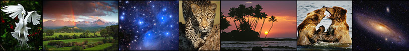
Keys to the colors in Figure 1 are the pink/magenta of hydrogen emission,
teal (greenish-blue) in the center of the nebula. The background
is mainly reddish-brown interstellar dust. There is also some faint
reddish-magenta hydrogen emission in areas of interstellar dust.
Normally, hydrogen emission is magenta due to red hydrogen alpha emission
at 656.3 nm, and blue hydrogen-gamma (434.1 nm) and hydrogen-Beta (486.1 nm).
Oxygen emits at 500.7 nm which is teal. When oxygen and hydrogen
emission lines combine we can get a mixing line from magenta to teal,
and that includes blue and purple-blue, which is also seen in the image (above the teal at the center of M8).
As the interstellar dust thins, it too will not change color significantly,
meaning it will not change to green or blue. If the interstellar dust gets
very thick it can turn a deeper reddish-brown.
Now that we have an understanding of these basic astrophysics principles.
let's work on Figure 2 to create a stretched image. I'll use the
color preserving stretch that also subtracts skyglow. In fact, it is
ideal that these two steps go together, because it is easier to find
the correct solution.
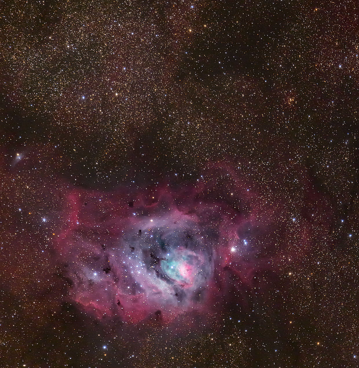
Figure 1. Messier 8 (M8), The Lagoon Nebula, final image. The image
is a stack of 19 frames, each 1.5 minutes, ISO 1600, with a 500 mm f/4 telephoto lens
and a stock digital camera. Only 28.5 minutes total exposure time.
Sky brightness = 21.6 magnitudes / sq. arc-second, Bortle = 4.
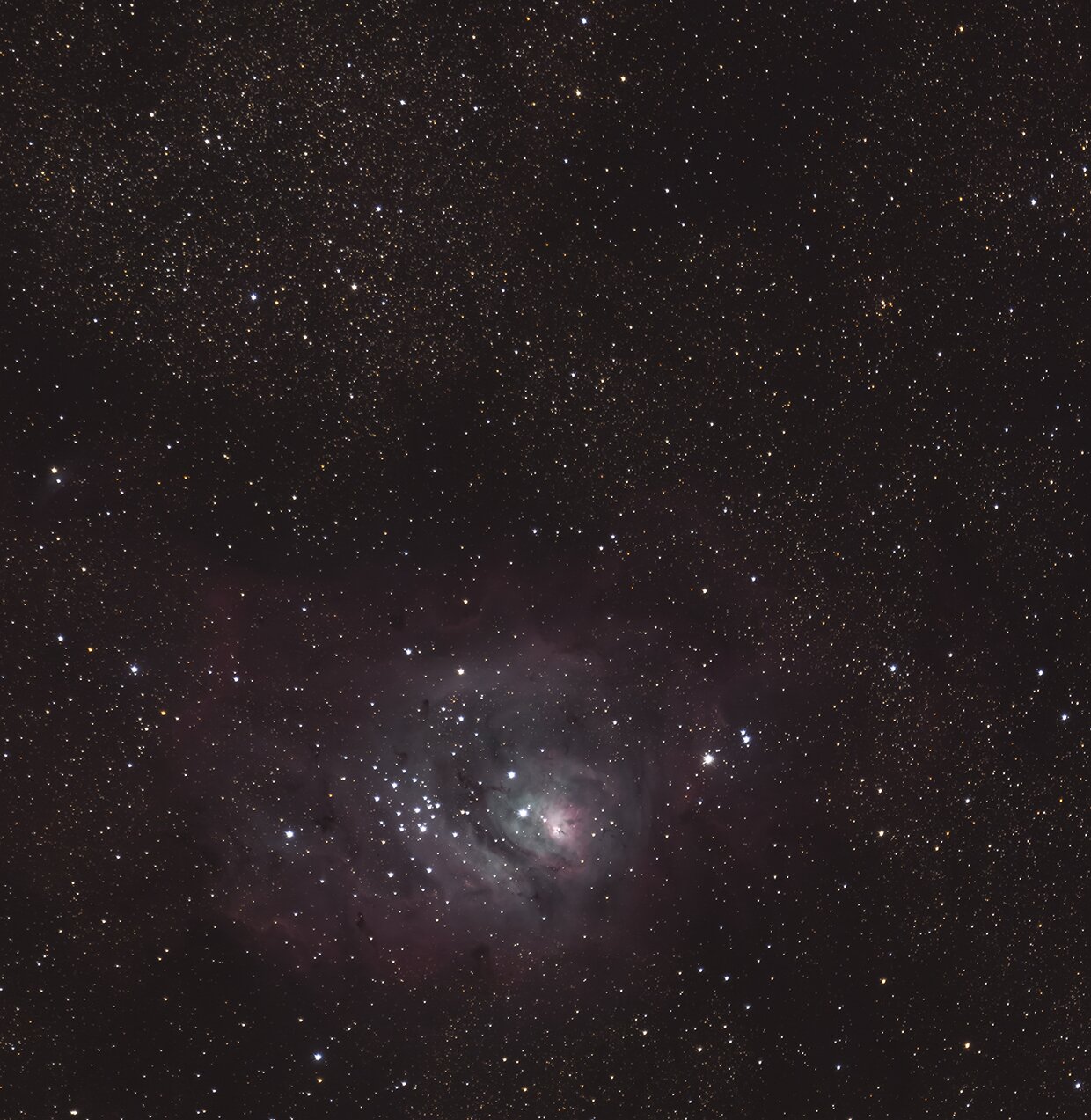
Figure 2. M8 after raw conversion in photoshop, and
stacking 19 images in Deep Sky Stacker.
An Example Black Point Error
I'll start with a modest stretch, rootpower = 4, shown in "Command 1" below.
Commonly taught on the internet is to align the histograms.
The skylevelfactor = 0.6 comes close to aligning the histogram peaks.
Command 1 also includes the parameter -plots which shows a histogram at
each step of the stretching and sky subtraction steps.
Stretch with the command:
rnc-color-stretch m8-500mm-09-04-2021-acr-IMG_0944-63-av19-0.33x-c2.a.tif
-rootpower 4 -scurve1 -setmin 20 20 20 -skylevelfactor 0.6
-rgbskyzero 6000 6000 6000
-obase m8-500mm-09-04-2021-acr-IMG_0944-63-av19-0.33x-c2-rs4-sc1-sm20-z6k-slf.6
-display -plots
(Command 1)
The first cycle with the sky subtracted but before the image was stretched is
shown in Figure 3 after two passes of estimating the sky background. Next the image
is stretched image and after pass 2 sky subtraction, the histogram is shown
in Figure 4. We see in Figure 4 that the histogram peaks are reasonably closely
aligned. The black point is pointed to in the Figure, the 0.6 level. At intensities above
that point (to the right on the horizontal axis), the low level intensities,
the histogram peak area, being aligned, means these intensity levels appear grey.
At intensities below the 0.6 black point set level, we see the histograms diverge,
with red lower (to the left) of green and blue. This means that fainter
levels are turned green/blue. The final stretched image using Command
1 is shown in Figure 5a.
Depending on your monitor, you may be able to see that the faintest parts
of the image are green and blue. Stretching the image a little more,
we see the result in Figure 5b. Now we see that the faint parts of the
image have indeed been turned green and blue. The green and blue colors
in the faint areas is due to processing and are not real.
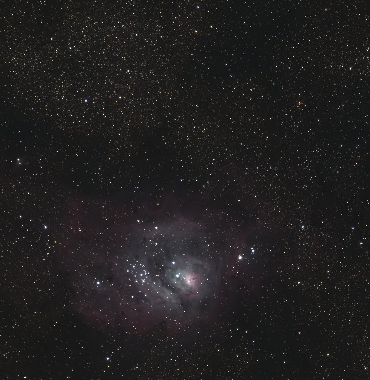
Figure 3. Image from Figure 2 after sky subtraction by rnc-color-stretch, but before stretching.
Note that the background color has changed, less red.
Figure 4. Histogram from the image in Figure 3 but after the stretch (rootpower 4 stretch).
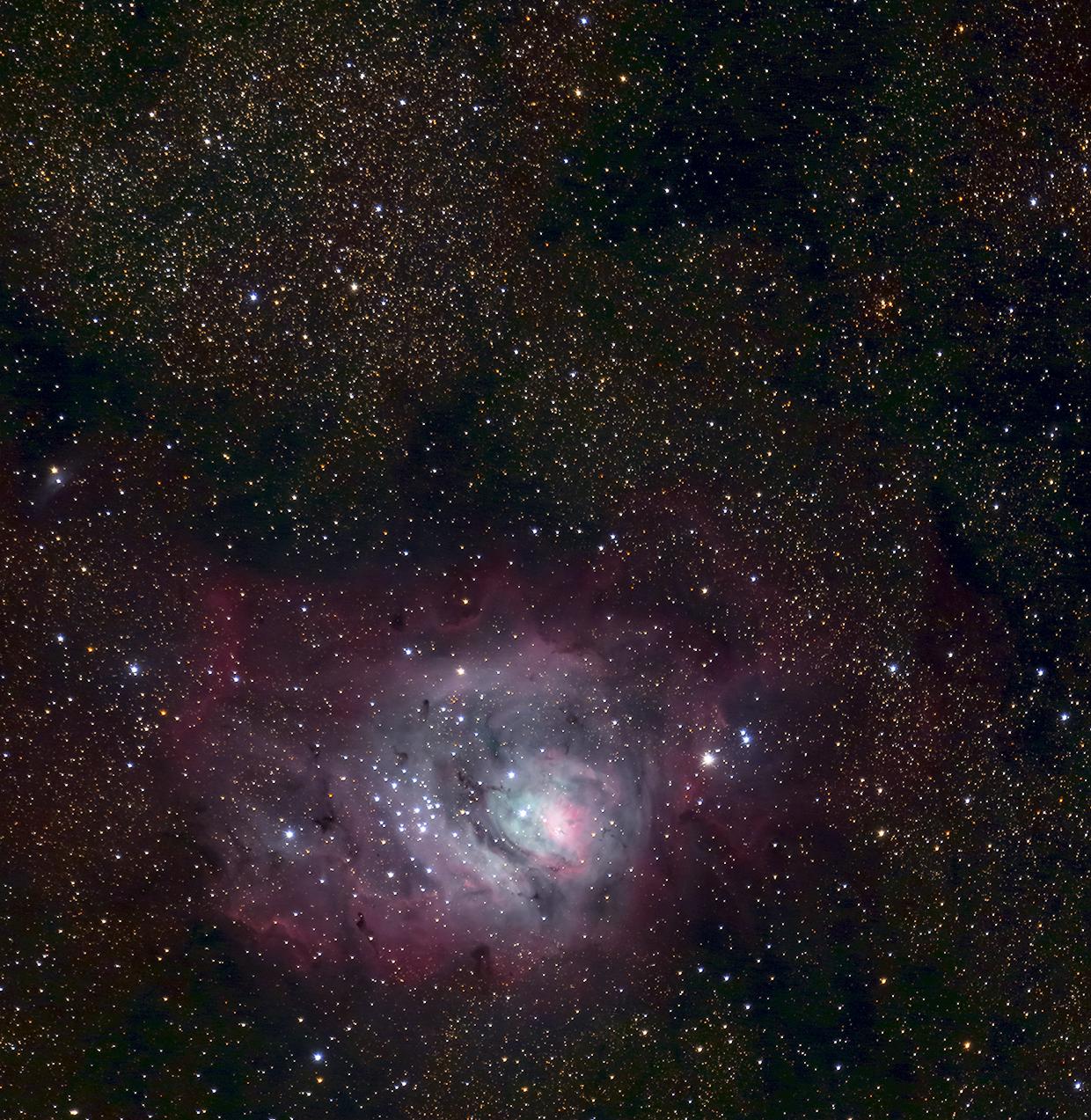
Figure 5a. Final stretched image from the stretching program (before color space assignment)
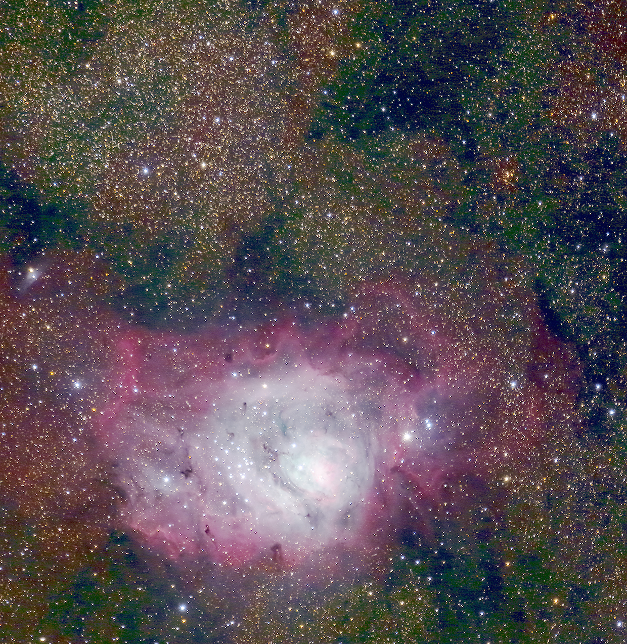
Figure 5b. Image from 5a stretched with curves tool in a photo editor to show
the low level color. We see a color shift, e.g. near the top center, red area shifted to green
then blue to the right of the red area. This is due to incorrect black point selection.
A solution is to reduce skylevelfactor. Reducing it to 0.01 should help.
The histogram peak is already reasonably dark sky, and a level 0.01
(1%) lower that the peak (this is 0.01 below the peak on the vertical scale).
For brevity, the image after stretching is not shown, but the histogram is shown in
Figure 6. There we see that that lower left part of the histogram still is
not aligned, and in this case green shows a higher intensity. This means that
the darkest parts of the image will still be color shifted.
The "internet" solution is a green reduction step. That is a band-aid that
may cover up the problem, and not necessarily result in correct colors.
Reducing green will turn those green areas blue, which is also not correct.
The next step will be to restrict the histogram to examine only a dark
part of the image. The histograms in Figures 4 and 6 cover the entire image.
Figure 6. Another run, same as above Comman 1, but with skylevelfactor = 0.01.
The solution is better, but still has a color shift problem.
Restrict the Black Point Selection Area to a Small Region
To restrict the histogram search for the black point, use a defined area (box)
covering a dark part of the image. To do this, rnc-color-stretch version 1.0
or later is required.
The image in Figure 2 was hand stretched with a curves tool in a photo editor,
and the result is shown in Figure 7. A dark area was selected and the upper left and lower right
coordinates were found. Those coordinates were included in Command 2 below. But just because
we selected a dark area does not mean that is is actually black. In fact, it isn't.
Nowhere in this image is there black space.
We need to find the color for the low level, and in so choosing, find the RGB level that causes no
artificial color shift. Once that level is found, then any stretch should show pretty consistent
color as the insterstellar dust fades into the dark area. In theory, going into the dark area
may be increased interstellar absorption so could also turn redder-brown, but there is no
astrophysical evidence for turning green or blue.
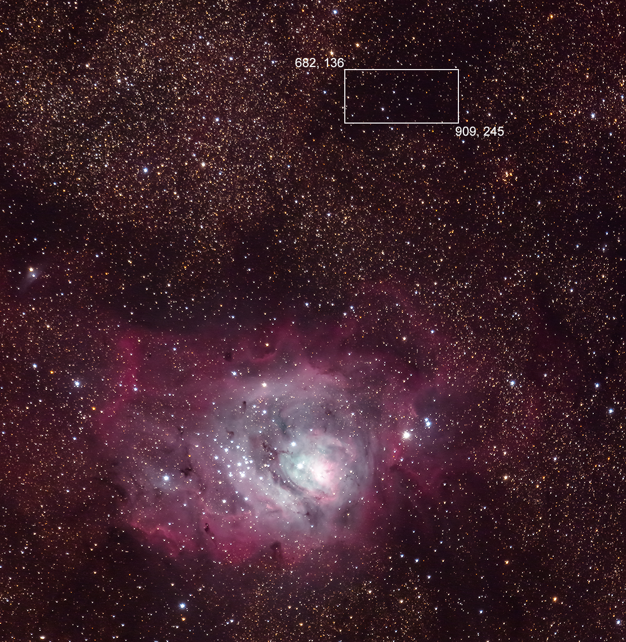
Figure 7. A quick hand stretch of the image from Figure 1 shows the darkest regions.
The box indicates the chosen area for establishing the black point.
This stretch was only to find a good region for the next step (the box outlined).
After a few iterations, it was found the rgbskyzero values of 4300, 3500, 2400,
(on a 0 to 65535 16-bit scale) works well and was added to the command (Command 2).
The stretched image with the sky subtracted histogram is shown in Figure 8.
Now we see that the RGB histogram peaks, and to the left side of the histogram peaks, that
red is to the right of green and green is to the right of blue, meaning
reddish-brown. The resulting stretched image for this pass of the
stretching program is shown in Figure 9a.
rnc-color-stretch m8-500mm-09-04-2021-acr-IMG_0944-63-av19-0.33x-c2.a.tif
-rootpower 4 -scurve1 -setmin 2000 2000 2000 -skylevelfactor 0.02
-histogrambox1 682 136 909 245 -rgbskyzero 4300 3500 2400
-obase m8-500mm-09-04-2021-acr-IMG_0944-63-av19-0.33x-c2-rs4-sc1-z432k-sm2k-hb1-slf.02
-display
(Command 2)
Figure 8. Histogram of the area in the box in Figure 7 after sky subtraction and established
the RGB black point = 4300 3500 2400 on a 0 to 65535 scale.
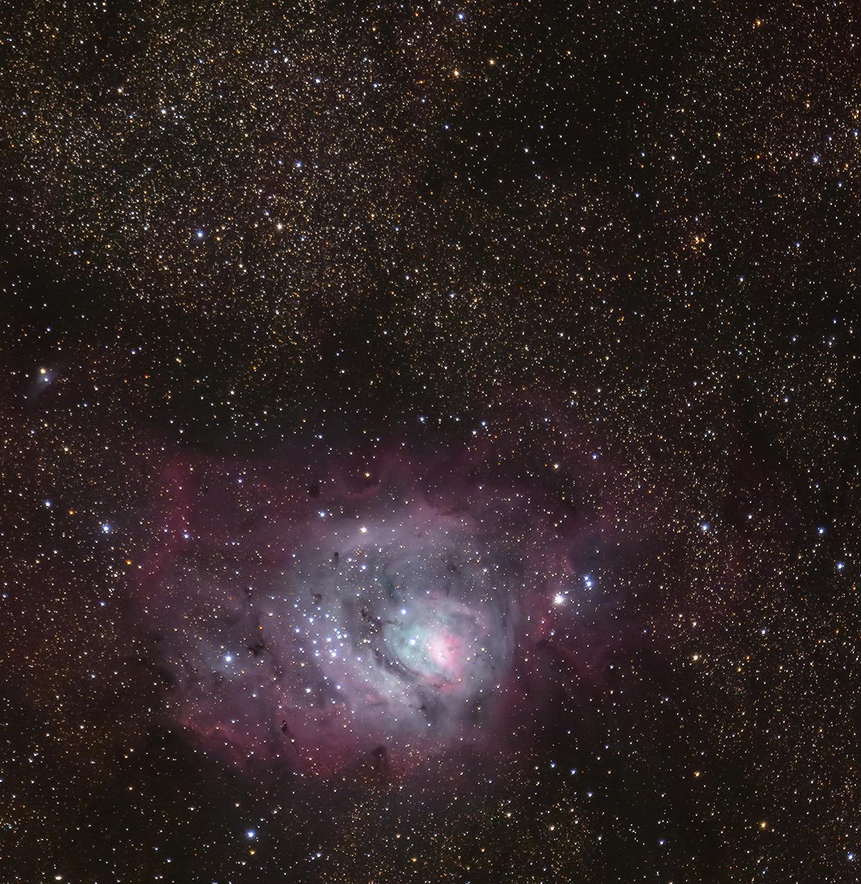
Figure 9a. Result out of the completed rnc-color-stretch using Command 2.
But the image does not yet have the correct color space assigned.
The output of the stretch program is shown in Figure 9a, above.
To confirm that the gradients into the dark areas do not have unusual
color shifts, the image on Figure 9a was hand stretched with a curves
tool in a photo editor. The result is shown in Figure 9b. Indeed, we
see that the colors are reasonably consistent going into the darker areas.
We do not have the ugly green and blue shifts like shown in Figure 5b.
There is some faint blue-green mottling but this is due to the raw conversion
and needing more exposure time for better signal-to-noise ratio of those faint
signals. Thus, the settings for the stretch (in Command 2) are reasonable for this data set.
After stretching and sky subtractions, a color analysis is performed.
Color recovery analyzes the color ratios of the sky subtracted image before stretching
compared to the after stretching and adjusts those ratios to match.
But it also limits changes in the ratios in an attempt to limit
effects from noise. After color recovery, the final histogram is shown
in Figure 10, and the final image from the stretch program that gets written
(Figure 9a).
The stretched Figure 9a image is not the final image. While it has
been stretched and skyglow subtracted, it does not have the color space assigned.
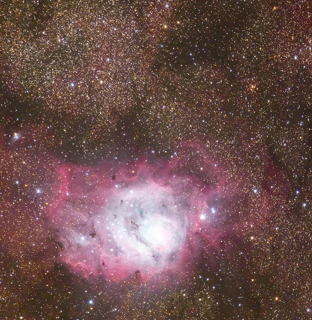
Figure 9b. Image from Figure 9a stretched with curves tool in a photo
editor to show the low level color. Here we see reasonably consistent
color of interstellar dust fading into the darkest areas. Compare to
the colors in Figure 5b. The color consistency shows that the black
point color and level was chosen reasonably well.
Figure 10. Histogram of the area in the box (Figure 7) after
stretching and color restoration, the image shown in Figure 9a.
The histogram of the final image (Figure 9a) from the stretch
program is shown in Figure 10. Remember, this histogram is only for the area in the
box shown in Figure 7.
The final step, when the stretching program is done, is to read the png file
into a color managed photo editor. The png file is on a 15-bit signed integer scale,
and photo editors assume a 16-bit unsigned integer scale. To change this, open
the levels tool and change the right level from 255 to 128. This brightens
the image by close to a factor of 2 (255/128 = 1.992). Next assign the color space (Adobe RGB
in this case), and suddenly, the color and contrast pop (Figure 11). Compare
Figures 9a with 11.
At this point one can consider the image finished. An optional step might be to
reduce the size of stars. That was done for the image in Figure 12.
Reducing star size alsop make nebula stand out better.
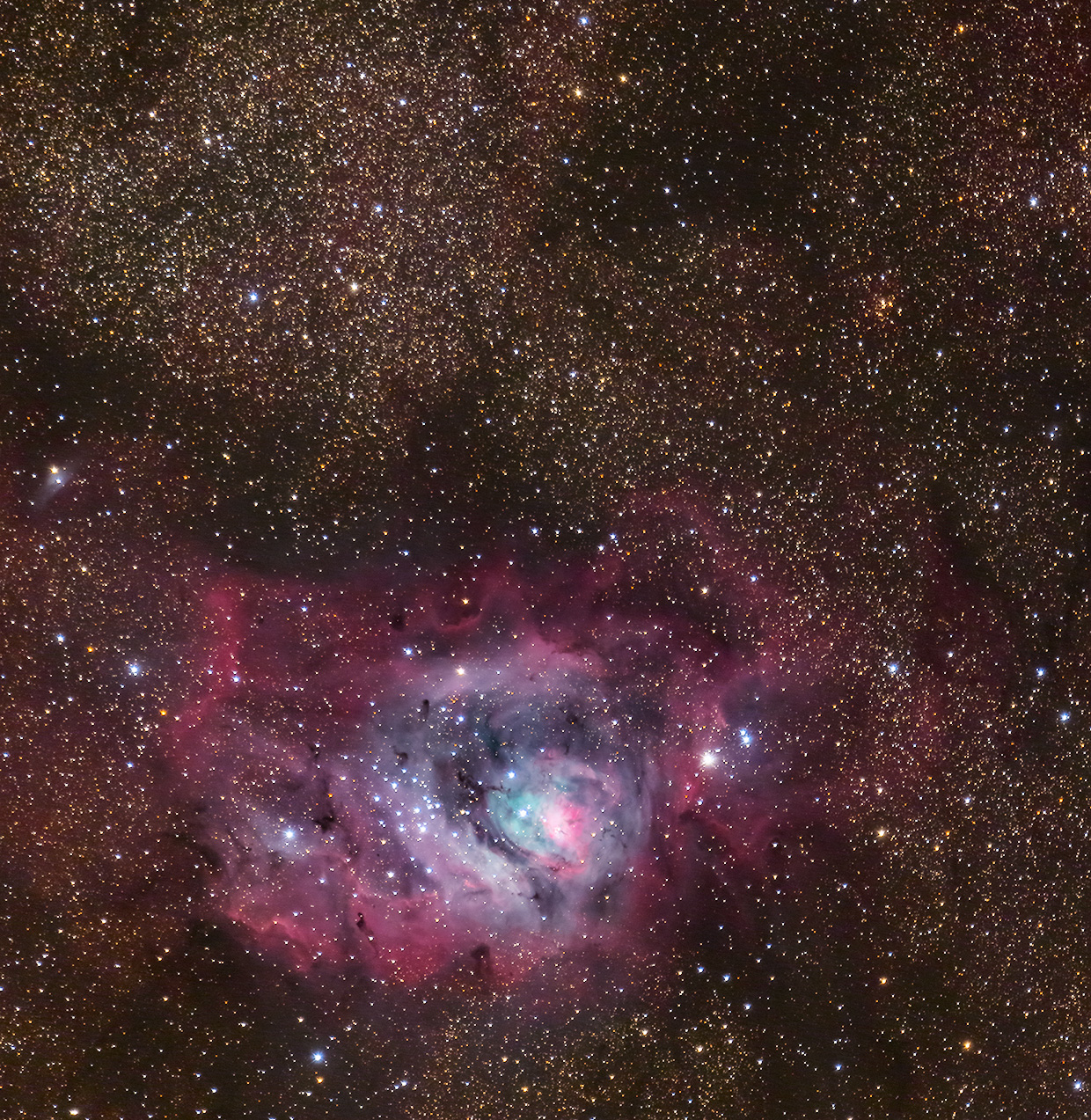
Figure 11. Image from Figure 9a with color space assigned, and a slight contrast boost added with
a curves tool in a photo editor. This could be considered final.
Figure 12. Final image. Image from Figure 11 with star reduction = 0.7 in ImagesPlus.
Summary of Processing steps
- 1) Raw convert (photoshop, rawtherapee, etc)
- Use daylight white balance
- Use lens profiles (includes a flat field)
- Output Adobe RGB, Rec2020 or your other favorite color space
- 2) Stack lights only (e.g. in Deep Sky Stacker; do not use autosav.tif file).
- 3) Choose a dark area in the image and get the coordinates of the bounding box.
- 4) Run rnc-color-stretch with the bounding box.
- 5) brighten resulting image from rnc-color-stretch in a photo editor and assign the color space.
- 6) (Optional) Touch up to taste in a photo editor, can include star size reduction.
Image Stretching Parameter Strategy
There are two stretching parameters to rnc-color-stretch: rootpower and rootpower2.
In general, I have found the best results with rootpower2 about 1/2 to 1/3 the amount
of rootpower.
For low signal-to-noise data, start small, with
rootpower = 2 or rootpower = 4 and no rootpower2.
If light collection is better but still low, start with
rootpower = 4 and rootpower2 = 2 and work up from there.
examples:
- rootpower = 2
- rootpower = 4
- rootpower = 4 and rootpower2 = 2
- rootpower = 6 and rootpower2 = 2
- rootpower = 8 and rootpower2 = 4
- rootpower = 12 and rootpower2 = 6
- rootpower = 20 and rootpower2 = 10
I have rarely found it necessary to go beyond the last one, 20 and 10.
If you are doing many iterations, I usually find it faster to reduce the image size
and perhaps crop it so that there is less data to process. Once I found a good set of
parameters, I'll process the full resolution image.
Make skylevelfactor as low as will run without errors. For example, try 0.01,
and work down until fails, e.g. 0.002.
The setmin parameter, e.g. setmin 2000 2000 2000 means if any data falls below
that leve, it is reset to the setmin value for that color. This prevents
dead pixels from making dark spots in an image. This could be made a fraction of
the rgbskyzero RGB values. For example, if rgbskyzero 4300 3500 2400, the
setmin values might be better set at 2000 1800 1500 or similar.
Notes:
Key to best results is to limit the histogram box to a darker part of the scene in the sky
(land is not relevant), and to make the skylevelfactor as low as possible. The default
skylevelfactor is 0.06, which means to choose the neutral point at 6% of the peak histogram.
If the histogram is the whole image, 6% may not be very dark. What can happen is that for areas darker than
that level, there can be a color reversal, e.g. making faint things can turn blue or at least less red than
they should be. A 2-level rootpower
helps mitigate this as the image is stretched by the first rootpower, then the skylevelfactor
is applied again, this time for the rootpower2 stretch. But lowering the skylevelfactor
from the 0.06 default also helps. If the histogram box is small, the histogram may look "ratty"
and the simple algorithm used to find the skylevelfactor may fail and an error results.
Start with a low skylevelfactor (e.g. 0.002) and work up until it works.
Or start at a little less than 0.06 and work down until it fails, then go back up a little.
Example error:
histogram sky level 0.002000 not found:
     channels: red 3743   green 2097   blue 0
     Thus, not sure what to do with this image because the histogram sky level is too low, quitting
          Try raising the skylevelfactor and/or
          Try raising the three rgbskyzero values.
          The input data may be too low.
Instead of just increasing -rgbskyzero values when you see the above or similar errors try increasing skylevelfactor.
The histogrambox1 needs to contain enough pixels to provide enough statistics to find the zero point.
For example, in the above image, I made a 2400 pixel wide image for testing parameters. A skylevelfactor
of 0.006 failed, but 0.008 worked. But when I ran tests on the full resolution image with the histogrambox1,
I was able to decrease the skylevelfactor to 0.001 because there were more pixels in the defined box.
The Night Photography Series:
First Published July 3, 2023
Last updated July 3, 2023.