ClarkVision.com
| Home | Galleries | Articles | Reviews | Best Gear | Science | New | About | Contact |
Astrophotography Image Processing
Using Modern Raw Converters
by Roger N. Clark
| Home | Galleries | Articles | Reviews | Best Gear | Science | New | About | Contact |
by Roger N. Clark
Learn modern practices, settings and processing tips for astrophotography here. Modern methods simplify astrophotography post processing and enable a better final result when using DSLRs for Astrophotography.
The Night Photography Series:
Contents
Introduction
Simpler Modern Methods for Astrophotography Image Processing
Processing Comparison
Conclusions
Other Examples
Appendix: Controversy
References and Further Reading
Traditional processing of astrophotos is complex and includes:
** The step between 13 and 14 is a needed calculation with digital cameras if one wants natural color, or even some decent looking color! The Bayer filters in a digital camera are not perfect matches to the color response of the human eye. For example, the red filters may allow blue and green light through. When digital camera raw data are converted into a color image, e.g. the jpeg conversion in the camera, or the conversion in a modern raw converter, corrections are applied to compensate for the out-of-band response of the color filters. This is done by a color correction matrix and the process is described well in this Cloudy Nights Forum thread. The thread shows that before the color matrix application, the colors are muted. The typical astro software as of this writing does not apply the color matrix correction. Thus after calibration and stretching, a saturation enhancement is typically done to recover some color. But that just amplifies existing color which includes the out-of-band response of the Bayer filters. The result is not necessarily natural color. The saturation enhancement will also amplify noise.
Figures in this article labeled Traditional Processing have been processed according to the above steps.
The above is quite involved, requiring a lot of attention to detail. But there is a simpler way that produces the same or even better results if you are imaging with a modern DSLR and does away with steps 2 through 11 plus the ** step, making post processing much simpler.
Modern DSLRs, post circa 2008 have on sensor dark current suppression. Modern raw converters have lens profiles that correct for lens aberrations, apply the flat field from a lens model, and ignore hot/dead/stuck pixels during raw conversion. Further, uniformity of modern cameras and the on sensor dark current suppression means there is no need to making dark or bias frames. The lens profiles mean there is no need for flat field measurements. This greatly simplifies astrophoto post processing. Further, during raw conversion, noise suppression on the raw data can be done, further improving the results. The technical know-how is greatly reduced, enabling more people to make great astrophotos. Steps 1 to 11 in the traditional processing method can now be done with a few quick and simple steps in a modern raw converter!
One key to astrophoto image processing is the image editor must work on at least 16-bit data or greater (like 32-bit floating point). If the image editor only processes 8-bit data, there is not enough precision to pull out the weak signals in the night sky.
This new method is not without controversy, because this is the age of the internet. Some people insist this new way is not correct and some have even declared that it is impossible to do some things with this method and that results with this method will be inferior. That is not true. Here are the steps in the raw converter:
Why the above is correct in light of traditional processing as as follows. The raw converter corrects light fall-off on the linear data, thus a flat field correction. The dark is irrelevant because it is suppressed by the camera (thus zero) in modern digital cameras with on-sensor dark current suppression. The airglow and light pollution gradients are subtracted in post processing after raw conversion, much like traditional processing.
Example settings in photoshop CS6 are shown (see up to Figure 5) here: Raw Processing Example and in other articles in this astro series.
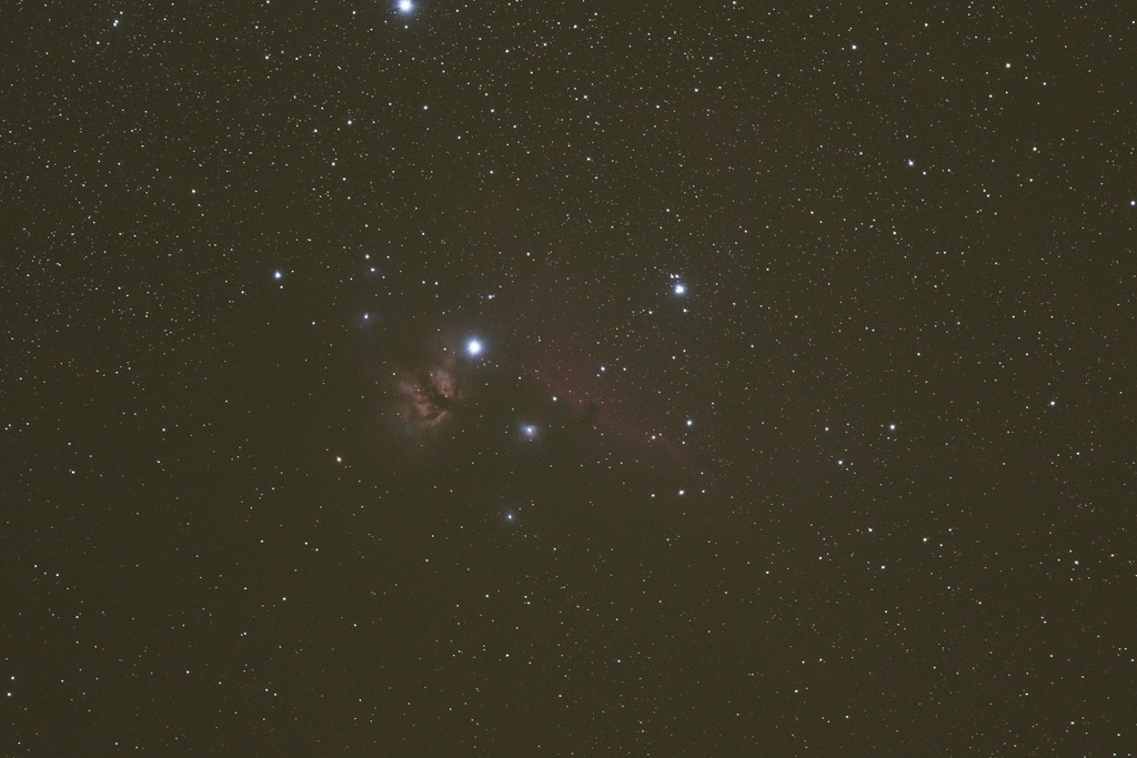
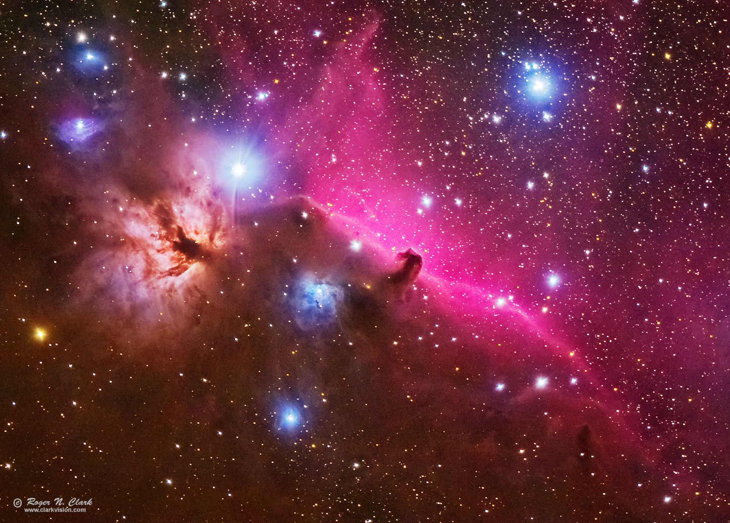
To show the difference between the traditional processing methods and the modern way, doing a lot of work in the raw converter, I chose 9 one-minute exposures on the Horsehead nebula made with a Canon 7D Mark II 20-megapixel digital camera and 300 mm f/2.8 L IS II lens at f/2.8. I chose 9 frames because 9 minutes of exposure is not really enough exposure time on this subject, so will show the noise differences between the methods.
A single one-minute exposure is shown in Figure 1a. Note the corners are darker than the center. This is due to light fall-off (vignetting). If such an image were stretched to bring out the nebula, the result is poor, as illustrated in Figure 1b. It should be apparent from these two Figures that astrophotos need good calibration for light fall-off. Note too, that the image in Figure 1b shows excessive noise. This is due to insufficient exposure time collecting too little light. Most of the noise seen in the image is from low light (photons); the signal-to-noise ratio is the square root of the total photons collected. The solution is to make more exposures and combine them in a process called stacking. In theory, one could do one long exposure, and people did that in film days. But an astrophoto can be ruined by airplanes and satellites making streaks through the image. The alternative is to make many shorter exposures, and stack them with a method that rejects one-time events like pixels with a satellite track. Stacking increases the signal-to-noise ratio. Compare the image in Figure 1b to the images in Figures 3 and 5 to see the positive effects of stacking.
I converted one copy of the raw files linearly and did a traditional processing method on the set using darks and flats. The darks had the same exposure time as the lights, so no bias frames were needed. A total of 100 flat frames were averaged so that noise from dark frames did not contribute significantly to the processing. Similarly, the 20 flat fields were averaged and smoothed so noise did not contribute significantly to the processing. With a second copy of the raw files, I converted them in Photoshop CS6 using the modern method described above.
Next, I aligned each set of 9 images in ImagesPlus and then combined them using the sigma-clipped average method using default settings. I show the combined average of the modern method in Figure 1. The traditional method image looks the same except that it is much darker with only the brightest stars apparent. Note the small dark edge on the image in Figure 1 (right and bottom sides). That is due to the alignment process and some small shifts between exposures. That dark edge was cropped out of both images.
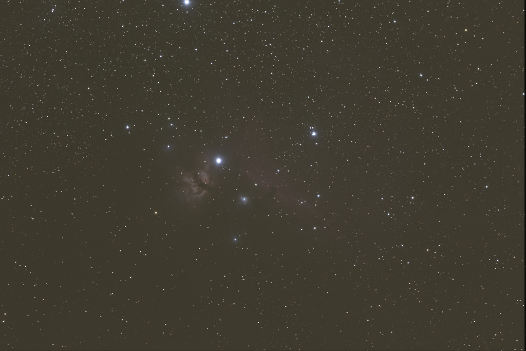
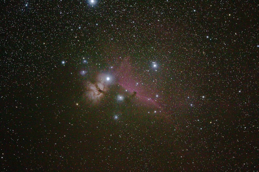
Next, I stretched the images to produce a reasonable output, subtracting and suppressing the airglow signal to pull out the weak signal of the nebulosity. As each image that I started with had a different stretch, the final result is close but you may perceive small differences in brightness and color balance. Ignore those, as they are not important for the comparison. The result of the traditional processing is shown in Figure 2, and the modern processing in Figure 3a with simple stretching with a curves tool. All stretching to increase brightness compresses the high end and loses color. To subtract the airglow and light pollution and brighten the weak nebula signal, I only used the curves tool according to the methods here: Night Photography Image Processing.
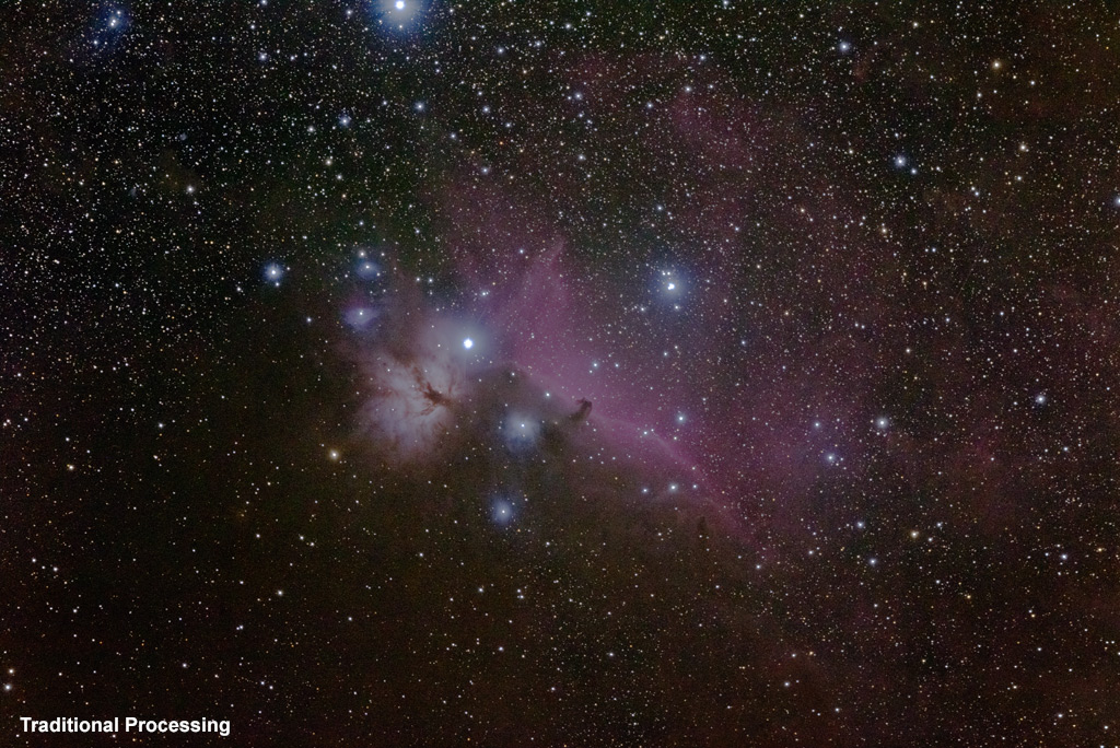
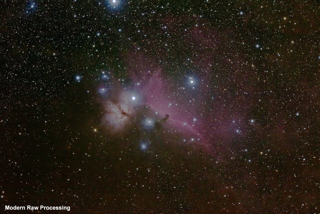
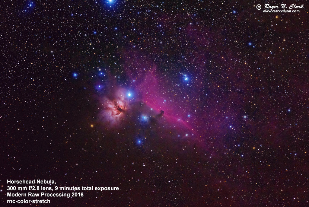
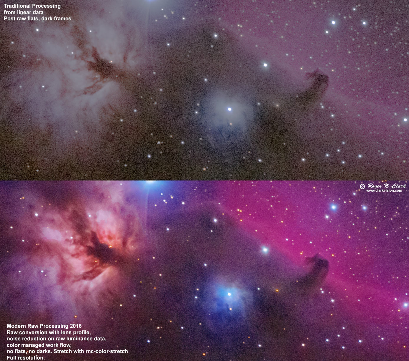
It should be apparent that the two methods illustrated in Figures 2 and 3a can produce very similar results. But the above images are greatly reduced. With newer stretching methods developed in 2016, the result in Figure 3b can be made with less effort and lower noise due to no need for saturation enhancement. The full resolution detail in the Horsehead region is shown for traditional and new methods in Figure 4. It should be clear that the modern processing method (bottom panel) shows great detail, better color ad less noise. Overall, I would rate the modern processing image the better of the two.
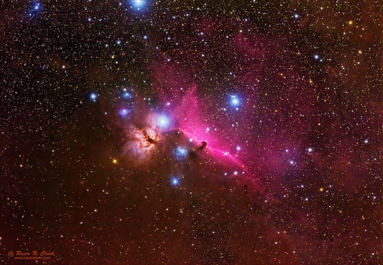
Of course, the best way to reduce noise is to increase exposure time. Figure 5 shows the Horsehead nebula with 70 minutes of exposure, recording extremely faint nebulae. The nine images used in the above comparison were from the set of 70 used to make the image below. The processing steps above are a good starting point for further processing, including additional noise reduction and image deconvolution to improve detail. Figure 6 illustrates a completed image where Richardson-Lucy deconvolution was applied in multiple steps (using 7x7 and 5x5 Gaussian profiles in ImagesPlus applied to brighter parts of the image, including stars). See my series on Image Sharpening for more details.
The use of modern digital cameras with on sensor dark current suppression (that means on-sensor dark frame subtraction during the exposure!!), combined with modern raw converters that use lens profiles (that means flat field corrections on the linear raw data) and reading the hot/dead/stuck pixel list from the raw file to correct bad pixels means astrophoto image processing is simpler, producing a better result than traditional methods. The example shown here used a top quality lens. If the lens had more aberrations, like chromatic aberrations, modern raw converters will correct that and can also improve other aberrations, making the difference between traditional and modern processing even greater.
Here are other examples on the internet where I have shown the method to others using their data. In each thread, see my posted results compared to other methods in the thread.
Orion, 30 100-second exposures with 85 mm focal length lens at f/4. My effort is on page 2.
This is the age of the internet, so someone is bound to object, some quite vocal. Usually someone fails to account for some practical factor (either the author of the method, or the critics). One of the main objections to the method described here is is that it is mathematically incorrect to subtract the sky signals from stretched images out of a raw converter with the standard tone curve, or a variation on it. The critics say one must only subtract the sky (light pollution and airglow) from linear data. Light pollution and airglow are added light, so it is proper to subtract it if one wants to remove it to reveal the beauty of deep space objects like galaxies and nebulae. First remember that this method of using a standard raw converter, and applying a tone curve has many advantages, including lens profile corrections to produce sharper images, noise reduction at the raw data level for less noisy images, faster post processing with no need for flat field and hot pixel corrections, and with modern cameras, no dark frame subtractions. This method is to produce a nice photo and is not for precise photometry.
The illustration above in Figure 4 illustrates little difference between the traditional method and the new method, and that the new method has not produced some bizarre artifacts that the internet ranters claim.
So how bad is the problem of subtracting sky on tone curve data? First thing to remember is that the tone curve applied to digital cameras is not a simple gamma function as is commonly cited on the internet. The function is shown in Figure 7a where the blue points are real data from a digital camera where the image was converted to a linear 16-bit tiff image and converted with a tone curve applied. The blue point in Figure 7a are tone curve data on the vertical axis. versus linear data on the horizontal axis. The plot is log-log to show the response over the full bit range of the camera data (the human eye also has a log response to light). Important to note is that the left half of the graph shows the data following a straight line. That line is Gamma = 1 thus linear (the slope is 1). This basic fact has important implications on why this method works and does not produce the horrible artifacts the ranters stomp their feet and throw tantrums about.
Most people understand that when you subtract a small number from a large number, the result is still a large number.
The typical astrophoto has the sky brightness in the left half of the graph in Figure 7a. This means that the data are linear so when you subtract sky, the result is "still correct math" which the ranters say is being violated. As scene brightness increases, and the non linear effects of the tone curve kick in, but the departure from linearity is at first slow, so the subtraction from linearity is not large and the "data destruction" the ranters claim never happens. As the signal gets larger and the tone curve non linearity kicks in stronger, one is subtracting a small number from a relatively large number and the result is still a large number little different from the original value so again no horrible consequences that ranters claim. The bottom line is that the subtraction of the sky signal from tone mapped image data method works because the tone curve is linear at low signals where sky would be a larger fraction of the signal and as intensity rises the subtraction is a small fraction of the intensity (linear or tone mapped data), so it doesn't matter if the data are tone mapped or not.
It is a very simple concept with quite simple math: subtract big numbers from little numbers and still get big numbers.
In practice, however, there is a positive side effect of the sky subtraction from tone mapped data. At the high end, the proportion of sky increases, meaning more is subtracted than would be if the data were linear, even though as discussed above and below it is only a few percent different. The positive aspect is that it increases contrast in the higher intensities! This is generally good because astronomical images are often low in contrast and this method of boosting contrast has no detrimental side effects (like saturating bright regions when using a contrast enhance slider in an image processing tool). So not only are there no "data destruction" side effects as ranters claim, there is positive result making images appear better than if linear processing only were done.
Technical Details. The tone curve is a variable gamma function of the form:
DN = CDN * b * (1/d) ( (CDN/c) 0.5 ) (eqn 1)
Where DN = the output Data Number, CDN = the input linear Camera Data Number, b and d are constants where b ~ d, and c is a constant usually set to near the maximum value. For example, for a 14-bit camera, c ~ 16383, for an 8-bit image, c ~ 255, and for a 16-bit tiff, c ~ 65535. The constants b, and d are around 10 to 12 and b ~ d. These are approximate because the high end gets scrunched, so setting c slightly different than the max tune that scrunching at the top. This page shows the shape of the data in Figure 7a in more detail: Dynamic Range and Transfer Functions of Digital Images and Comparison to Film. Also note that at the low end of the intensity range, CDN/c becomes small, much less than one, and that makes the exponent small so the factor (1/d)small exponent approaches 1.0 for small signals and the response is linear. The linear response is shown in Figure 7a. Whenever the signal is at about half histogram or less, the output tone-stretched data are in the linear regime.
See more on tone curves here, including many technical references.
In astrophotography, it is often recommended that one sets exposure time so that the sky signal appears well separated from the left side of the histogram on the camera to be sure no data are truncated. Further, the recommendation is that the sky histogram peak appears about 1/4 to 1/3 of the way from left to right so that the exposure is well above camera read noise (these recommendations were made when read noise was much higher than today's cameras which now typically have read noise under 3 electrons). In any event, it is an extreme case if you use such levels. On a 14-bit camera, that would be 16383/3 or 5461 on the stretched scale. A CDN value of 1000 gives almost exactly that value, 5658 from equation 1 with b=16383 for a camera with 14-bit output.
That 1/4 to 1/3 of the histogram is basically the left half of the plot in Figure 7a. That keeps the data in the linear range, so regardless of the trolls, who complain about improper math, the equations still work. That is ironic, because one can find online the trolls using improper math to claim all this doesn't work: they use a pure gamma=2.2 function, but the data are not a gamma=2 function at the low intensity end of the data.
The effect of subtracting sky on the tone curve stretched data is illustrated in Figure 7b. As above, the sky signal was CDN= 1000. The Canon 7D2 was modeled to derive photon counts. I use the Canon 7D Mark II camera at ISO 1600, and the camera gain at that ISO is 0.168 electrons/CDN. Thus a sky value of 1000 CDN is 1000 *0.168 = 168 photons. Next I computed the linearly corrected sky using rigid math, then used equation 1 to compute the tone stretched response of a subject plus the sky of 168 photons, subtracted a sky on the tone curve stretch then computed the ratio of tone-curve corrected data divided by the linearly corrected data, shown in Figure 7b. Also shown is the +/- one standard deviation noise envelope of the photon signal. It is clear that the error of applying a subtraction to tone curve stretched data amounts to only a few percent and the error is smaller than the noise envelope from photon noise. The actual noise envelope for the data is larger because one would add camera noise to the photon noise. Thus, the error produced by the nonlinearity is negligible for producing nice astrophotos. It also demonstrates that one could also use such data for photometry if one only needed accuracy to a few percent. Indeed, the errors are so small that traditional processing (linear signal - sky) versus new modern processing methods have characteristic curves that overlay very closely, as shown in Figure 7c.
Note any stretching of the image data using curves, levels, or math functions is the application of a tone curve. If you have ever changed the black point in the stretching of the data after any application of an such functions, it is a subtraction of the nonlinear image data because after the tone curve application, the data are no longer linear. You have now done the very thing the critics of the methods above object too. But this is the standard practice in image processing. Sure if we wanted to do precise photometry such manipulations are inappropriate, but we are SIMPLY TRYING TO PRODUCE A NICE PHOTO that shows good contrast. The controversy is a non issue.
There is another positive side effect at play as discussed above. By subtracting a constant from tone stretched data, whether it be sky or just some random constant, what the trolls complain is improper math, let's look at the effect on the brighter parts of the image. Because the data are tone stretched, the brighter intensities are compressed. That means that they are not as high in intensity as if the data were linear. Thus we are subtracting a too much from the tone stretched high intensities. Oh the horrors! The math is not linear! Well, guess what the side effect is: it just increases contrast in the brighter parts of the image. This is something one usually needs to do with low contrast images anyway. So the side effects are positive for producing a more interesting image. The trolls are now screaming and yelling. So what? Let them scream.
One trolls says all of the above is wrong and that the tone curve is a simple gamma function. A simple gamma function used in monitors has the form (with gamma = 2.2):
DN = CDN (1/2.2) (eqn 2)
Math students will immediately recognize that this function will plot as a straight line on a log-log plot as in Figure 7a, and thus will not match the data from tone curve applied data. This is shown in Figure 8. Basically, the ranter who complains the method is all wrong because the tone curve is a simple gamma function is completely wrong.
Indeed, as discussed in Digital Image Processing: An Algorithmic Introduction Using Java By Wilhelm Burger, Mark J. Burge pages 76-78, the tone curve is separated into segments with the lower portion being linear (see equations 5.33 and 5.34 on page 78 of Burger and Burge). Case closed on the ranter.
Well, the troll insists DCRAW is the gold standard and the output of DCRAW is a gamma = 2.2 tone curve. Figure 9 shows the default DCRAW tone curve, and the lower half of the histogram (the lower half of the plot) parallels the linear line (gamma = 1.0), which means the output is linear over that range, and is closer to the gamma=1 range over the whole plot than is the gamma = 2.2 line. DCRAW output approaches the gamma 2.2 slope at the highest intensities.
How common is the digital camera "standard tone curve?" Figure 10 shows another way to plot the data and compare it to a gamma 2.2 function. Of note is a gamma 2.2 function is concave over the entire data range, while the tone curve data follow a convex trend at high intensities and decrease faster than a gamma 2.2 function at low intensities. Dpreview.com plots data for many cameras in this fashion. For example, compare the tone curves for many cameras here on dpreview.com.. On the dpreview site, the Canon tone curve for the 6D is very close to the blue points in Figure 9. Comparisons to other manufacturers and numerous camera models show very close tone curves, none of the ones I have looked at follow the gamma 2.2 shape. There is some variation in the upper end of the tone curves between manufacturers, but more uniformity at the low end where the tone curve is linear. Thus, the blue data points are representative of many camera models and manufacturers, especially the lower half of the plot. Again, this means that the low end of the tone curve is linear and the sky subtraction method on tone curve data and new astrophoto image processing methods presented here works well for many cameras.
The digital camera tone curve data are shown in an all linear graph in Figure 11. Here we see that at the typical sky level, the digital camera tone curve is linear in the local region of typical sky levels in an astrophoto and that any departure from linearity is much smaller than the photon noise. As signal increases the percent error is small because one is subtracting a relatively small number from a much larger number and any error from nonlinearity is small and within photon noise (Figure 7b). Thus, the method produces no bad artifacts as charged by online trolls.
Digital Camera Tone curves, Camera Response Function, Opto-Electronic Conversion Function (OECF)
Contrary online trolls insisting that the digital tone curve data from raw converters who say the tone curve is a gamma 2.2 function, sRGB, function or BT.709 function, the data presented above prove otherwise. So do many scientific papers on the subject:
Garcia JE, Dyer AG, Greentree AD, Spring G, Wilksch PA (2013) Linearisation of RGB Camera Responses for Quantitative Image Analysis of Visible and UV Photography: A Comparison of Two Techniques. PLoS ONE 8(11): e79534. doi:10.1371/journal.pone.0079534
http://paperity.org/p/60767995/linearisation-of-rgb-camera-responses-for-quantitative-image-analysis-of-visible-and-uv
"camera responses... successfully fitted the entire characteristic curve of the tested devices, allowing for an accurate recovery of linear camera responses."
"Linear responses from consumer-level cameras can be recovered by fitting a function to a plot of camera response versus incident radiance, the Opto-Electronic Conversion Function curve (OECF), and subsequently inverting the fitting function via analytical or graphical methods, or look-up tables (LUTs) [19]. Polynomial, power and exponential functions have been previously suggested as fitting functions [20,21]."
"Here we compare the use of (parametric) cubic Bezier curves and biexponential functions for characterizing two camera models"
"In spite of being sensitive to different regions of the spectrum, the OECF curves of the two tested cameras present a notable similarity in their general form. This result indicates a close likeness between the gain functions applied to the sensor response of the two cameras."
http://profs.info.uaic.ro/~vcosmin/licenta/lucrari_licenta_in_desfasurare/HDR/ebooksclub.org__High_Dynamic_Range_Imaging__Acquisition__Display__and_Image_Based_Lighting.pdf
"Assuming an sRGB response curve (as described in Chapter 2) is unwise, because most makers boost image contrast beyond the standard sRGB gamma to produce a livelier image. There is often some modification as well at the ends of the curves, to provide softer highlights and reduce noise visibility in shadows."
http://www.ee.columbia.edu/ln/dvmm/publications/PhD_theses/jessiehsu_thesis.pdf Image Tampering Detection For Forensics Applications PhD These, Columbia U, 2009
"Camera Response Function (CRF), pages 37-38: The CRF is often denoted as a single-variable function R=f(r). Although different manufacturers may produce different dynamic ranges of irradiance r and brightness R, without loss of generality, both r and R are assumed to be between [0,1]. Some popular parameterized models are listed as follows:"
PCA-based empirical model of response (EMOR) [31]
Single-parameter gamma function R=f(r) = r^a0 [32]
Polynomial R = f(r) = SUM n=0 to N r^Bn [33]
Generalized gamma curve model (GGCM) R =f(r) =r SUM i=0 to n ai *r6^i [34, 35]
"Generally, more parameters lead to more accurate representations of the CRF with the drawback of increased complexity. Therefore one should choose an optimal model considering the trade between approximation accuracy and computational complexity. A comparison among these models is given in [34] and [35]. The EMOR and GGCM have been shown to approximate CRFs better than the gamma and polynomial models."
the above reference [31] is:
[31] M. D. Grossberg and S. K. Nayar. What is the space of camera response
functions? IEEE Conference on Computer Vision and Pattern Recognition, 2003.
http://www1.cs.columbia.edu/CAVE/publications/pdfs/Grossberg_CVPR03.pdf
"a camera's response function can vary significantly from an analytic form like a gamma curve."
Thus, the internet trolls are wrong (again). Of course, even faced with real data (e.g. the blue points in the plots above) and scientific references they still insist the tone function is an sRGB, BT.709 or Gamma = 2.2 function.
Yet another complaint is doing deconvolution sharpening on the tone stretched data. Of course the other set of photographer trolls complain and say you should only do sharpening at the very end after all stretching (see my articles on sharpening). The astro trolls say sharpening must be done on linear data only. They say the data must be linear and point to the distortions over the intensity range of the image with the tone curve applied. If I had some detail going over the whole range of intensities, it would be high contrast and wouldn't need sharpening. Sharpening is needed to improve the low contrast things in the scene. That means small intensity ranges. Again the trolls are blinded by a full intensity range tone curve, and not seeing the fine low contrast details. When I'm trying to coax out more detail in a dark lane in a galaxy arm that may range from DN 5000 to DN 5100, it matters little what the non linearities are from 0 to 65000. Over that short range, it can be considered linear to a good approximation. Indeed, deconvolution sharpening works well on tone-stretched data. The trolls also complained that one can't do more than one sharpening pass with different blur functions. I challenged the troll complaining about my sharpening methods to show me how to do it better using a single run of a single blur function with the examples on my sharpening articles, and months later he has not. The fact is that there is no one perfect formula for sharpening. I run multiple tests with different sharpening parameters. Noisier parts of an image can't stand as many iterations as higher signal-to-noise areas of an image. Multiple runs can be combined to apply more aggressive sharpening in parts of the image that have the signal-to-noise ratio. You are welcome to prove otherwise, but not by just ranting; prove you can get a better result and show how you did it.
Another controversy raised is the use of noise reduction before other post processing like stacking. Of course, the internet trolls simply declare it is not correct, but as usual offer no scientific papers to say why. See Understanding Digital Raw Capture Adobe.com for information on noise reduction during raw conversion. It is common in signal processing to filter data. Also see: Sharpening and noise reduction in Camera Raw.
Online arguments against noise reduction before stacking include detecting methane on Mars: "The best example I can give you is the detection of methane on Mars. Its signature (about 10 parts per billion), entirely indistinguishable from the noise in a single measurement, was only found after taking over 1700 measurements and stacking them, just as we take multiple subs. What do you think would have happened if the folks at ESA would've noise reduced the individual measurements and then stacked them?"
The Planetary Fourier Spectrometer (PFS) that detected methane on Mars, like all FTIR is apodized. That means the high end frequencies are reduced. Apodization in the Fourier domain is smoothing in the spectral domain (reference, see page 18 at: http://mmrc.caltech.edu/FTIR/Understanding%20FTIR.pdf. More information on apodization is at: http://www.shimadzu.com/an/ftir/support/tips/letter15/apodization.html. I was a scientist Co-investigator on the Mars Observer and Mars Global Surveyor TES imaging Fourier Transform Spectrometer. I also work with FTIR lab spectrometers and have dozens of published papers using such instruments (see my publications list in the about link at the top of this page). Every FTIR instrument I have used/analyzed data for was apodized. That means smoothing before coadding (stacking).
There are scientific papers in imaging research that do noise reduction before stacking. Here is an example of a peer reviewed science paper: Migliorini, A., J. C. Gérard, L. Soret, G. Piccioni, F. Capaccioni, G. Filacchione, M. Snels, and F. Tosi, 2015, Terrestrial OH nightglow measurements during the Rosetta flyby, Geophysical Research Letters, 10.1002/2015GL064485. In this paper, first the authors do noise reduction: "In order to remove high-frequency spatial noise, the cube image was cleaned using a median filter combined with a smoothing procedure, applied in the spatial direction while the temporal and spectral dimensions were kept unchanged." Next they do stacking: "Since it was verified that the emission is roughly located at about 90 km, we averaged a total of 300 radiance spectra collected between 87 and 105 km in order to increase the signal-to-noise ratio."
Another smoothing before stacking, this time of satellite data is described in Yale et al., 1995 Comparison of along-track resolution of stacked Geosat, ERS 1, and TOPEX satellite altimeters, J. Geophysical Research, v. 100,. 15,117-15,127. See page 15,119: "A low-pass Parks-McClellan filter, designed with the MAT-LAB© Signal Processing Toolbox, is applied ... This prestack filter is intended to suppress the high-amplitude, short-wavelength noi... Later, we show that these prestack filters do not attenuate signals ..." http://topex.ucsd.edu/sandwell/publications/63.pdf.
Another example of scientific smoothing is in signal analysis. An incoming signal at a certain frequency is sent through electronics that only select that frequency. That in fact is a standard procedure in infrared astronomy where source and background are alternately chopped back and forth and the signal sent through a phase lock amplifier, then digitized and averaged. Again, that means smoothing before coadding (stacking).
Yet another example of smoothing before stacking. Earle and Shearer, 1998, Observations of high-frequency scattered energy associated with the core phase PKKP, Geophysical Research Letters, vol. 25, 405-408. http://igppweb.ucsd.edu/~shearer/mahi/PDF/54GRL98a.pdf. See the section on data selection and stacking: "To eliminate signal-generated and ambient noise at low frequencies, the data are filtered to a narrow high-frequency band (0.4 to 2.5 Hz)." Then they say: "After filtering, we select an initial set of seismograms with good signal-to-noise (STN) for stacking."
For more detail on the math of noise reduction, see this article on smoothing from the University of Maryland. Note in particular, Figure 4 in that article. The profile in that figure 4 is similar to a star profile on the Figure 4 on this web page (the Horsehead nebula image above). Note the noise in the Horsehead image is very fine compared to the star diameters. Some smoothing reduces the noise enabling one to see the stars better, just like the example in the U. Maryland Figure 4. Another way to describe this is the noise in the Horsehead image is higher spatial frequency than the detail in the image, thus smoothing can reduce noise without strongly affecting the image content. This is an advantage of the high pixel density digital cameras available today.
Here is a paper on data reduction of the NASA Cassini spacecraft imaging system where noise reduction is done very early, even before dark subtraction: http://pds-imaging.jpl.nasa.gov/data/cassini/cassini_orbiter/coiss_0001/document/cisscal_manual.pdf
See page 8+, where it says "The steps discussed below are always performed in the same order that they are listed here" and the steps are: 1) LUT conversion, 2) Bit weight correction, 3) Subtract bias, 4) Remove 2-Hz noise (that means running a noise reduction filter), 5) Subtract dark, 6) A-B pixel pairs, 7) Linearize, 8) Flatfield, 9) Convert DN to flux, 10) Correction factors, 11) Geometric correction.
If you use a Bayer sensor camera (e.g. Canon, Nikon, Sony, etc. DSLR), when you demosaic, smoothing is done, even by the default algorithms. Typically a radius of about 5 pixels is commonly used in the demosaicking process. You can prove this yourself by converting to a fits or 16-bit tiff file with your favorite de-bayering program, and convert using DCRAW with no de-bayering. Next, extract and do statistics on one color channel, e.g. green pixels in an intensity smooth area in the DCRAW file, and the same pixels in the converted file. You'll see the converted file has lower noise. For the demosaicking programs I use, noise is reduced to about 2/3 the level in the original values. Thus the demosaicking algorithms are smoothing and the amount depends on which algorithms are used.
And then we have cameras, like Nikons and Sonys that do internal smoothing of the raw data. By the arguments here, one would believe that no one can produce even a good astrohoto with one of these cameras, let alone a great one. Clearly that is not the case. And can anyone really prove Canon doesn't do some form of smoothing internally to their raw data? Is any consumer digital camera truly raw?
The more sophisticated demosaicking algorithms allow the user to tune the filtering, like what I show with Adobe Camera Raw, ACR. With software like this, one simply trades spatial detail versus noise. In the examples I show, I do not believe any stars were lost. There are noise clumps in the demosaicked images from the other programs (not ACR) that could be mistaken for stars, and those images give far more false positives of faint stars. The smoothing in ACR allows the user to choose how much noise reduction to apply. So if your star sampling is not ideal, like a star fits in one pixel, one can't do much noise reduction. But if you have several pixels across a star profile, you can do more noise reduction. Done well, that does not destroy information, and can help bring out more information and can remain scientific.
The key to remember (especially for the internet trolls out there) is that the methods described here are to enable one to make pleasing photos by faster simpler methods than the traditional complex methods in astronomy. It is not to do ultra precise photometry (even though one could--one just needs to track the non-linear tone curve).
References and Further Reading
Clarkvision.com Astrophoto Gallery.
Clarkvision.com Nightscapes Gallery.
The open source community is pretty active in the lens profile area. See:
Lensfun lens profiles: http://lensfun.sourceforge.net/ All users can supply data.
Adobe released a lens profile creator: http://www.adobe.com/support/downloads/detail.jsp?ftpID=5490
More discussions about lens profiles: http://photo.stackexchange.com/questions/2229/is-the-format-for-the-distortion-and-chromatic-aberration-correction-of-%C2%B54-3-len
The Night Photography Series:
| Home | Galleries | Articles | Reviews | Best Gear | Science | New | About | Contact |
http://clarkvision.com/articles/astrophotography.image.processing
First Published January 6, 2015
Last updated April 16, 2019