ClarkVision.com
| Home | Galleries | Articles | Reviews | Best Gear | Science | New | About | Contact |
Sensor Calibration and Color
by Roger N. Clark
| Home | Galleries | Articles | Reviews | Best Gear | Science | New | About | Contact |
by Roger N. Clark
Producing natural, or at least consistent color from a digital camera requires multiple complex steps, some of which are skipped in the traditional astrophotography work flow. The basic sensor calibration that amateur astronomers talk about are the same steps needed to produce any image out of a color digital camera, including daytime landscapes, portraits, sports or wildlife photos. The traditional astro work flow will not produce good everyday color images, not even as good as an out-of-camera jpeg from a smartphone! I advocate a simpler modern method for astrophotography that allows one to produce very good images with a modest amount of time and equipment, with better color and a more complete calibration than done with a traditional astro work flow.
The Night Photography Series:
Contents
Introduction
Calibrating a Sensor and Calibration Characteristics
Sensor Calibration Data
The Calibration Equation
Reducing Noise Through Technology
Demosaicing
White Balance
Color Calibration Problem
Color Matrix Correction
Stacking
Stretching
Simpler Modern Work Flow
Image Signal-to-Noise Ratio with the Modern Work Flow
Example Comparisons of Modern vs Traditional Work Flow
Discussion and Conclusions
Appendix 1 Sample Images: NASA APOD and Images by Others Using My Modern Methods
References and Further Reading
People new to astrophotography are taught to obtain all kinds of data to calibrate their images, with terms like lights, darks, bias, flats, flat-darks, flat-bias, and to obtain many of each, all thrown into astro processing software that "calibrates" the data. The output then needs to be brightened and contrast improved to see an image of your target. Then, typically, other enhancements, including saturation enhancement (because the colors out of this process are not very good). Often taught are other processing steps like histogram alignment, or histogram equalization, that are actually destructive to color, shifting color as a function of intensity in the scene. In this article, I'll compare the astro work flow with everyday photography work flow, and show with less work how to make beautiful images with better and more consistent color.
The modern method that I describe uses modern digital camera raw converters to produce a color image, exactly the same as one would do for a daytime landscape image, or a portrait of a person. But astrophotography has an added problem: light pollution and airglow is an unwanted signal. It is like making a daytime landscape photo on a foggy day, but the fog is strongly colored and you want an image of a clear-day view with no fog or haze.
The calibration of a color digital camera image requires many basic steps, and the traditional astro work flow skips two critical ones. The steps include 1) bias correction, 2) dark subtraction, 3) demosaicing, 4) flat field correction, 5) distortion and aberration correction (optional), 6) white balance, 7) color matrix correction (critical, skipped by traditional work flow), 8) tone curve, and 9) hue (tint) correction (skipped by traditional work flow). Modern digital cameras with modern raw converters, like Rawtherapee, Photoshop, Lightroom and others, include all the calibration steps, including critical ones skipped by the traditional astrophotography work flow.
As a professional astronomer, I use many kinds of digital sensors, in laboratories, in the field, on telescopes, on aircraft, and on spacecraft, from the deep ultraviolet to the far infrared. The traditional work flow for digital sensors is accurate for producing scientific data at single wavelengths. I use the traditional work flow for producing scientific data, but this work flow falls short for producing visual color, and this has led to mass confusion on what the color of objects in the night sky actually are. Note, this is independent of artistic license. For example, if you, as a photographer want to color a lion image you made on the Serengeti blue, that is fine, just not reality, nor close to what people see visually and not what a typical digital camera will record. Even a cell phone will get reasonable color of that lion that is close to the colors people see visually for those with normal color vision. This article is not about producing scientific data; it is about producing color images of the night sky with colors as good as what a cell phone can get colors of a lion on the Serengeti, or a local zoo.
Also note that professional observatories most often do not image in RGB color with filters that cover the visual spectrum. The RGB filters in the Johnson UBVRI filter sequence cover more than the visible spectrum. The B filter includes UV and the R filter includes infrared. The Hubble telescope also does not have a RGB filter set to make color images that only include the visible spectrum. Astronomers use wavelengths beyond the visible spectrum to provide more leverage in scientific measurements, so B filters include ultraviolet and red filters include infrared beyond what we see with our eyes. As a result, images from Hubble and other professional observatories can't be used as color standards for objects in the night sky for visible RGB color.
Types of Noise First, let's discuss the types of noise from a digital sensor. Noise comes in two general ways: random and patterns.
Random noise is seen from several sources, including noise in the light signal itself, equal to the square root of the amount of light collected. The ideal system is called photon noise limited, and most of the noise we see in our digital camera images is just that: noise from the light signal itself. To improve the noise, the only solution is to collect more light, either by a larger aperture, or longer exposure time, or both. Light collection from an object in the scene is proportional to the aperture area times exposure time, and the noise will be proportional to the square root of the product of aperture area times exposure time.
Sensors also show random noise from reading the signal from the sensor, called read noise. After the sensor, the camera electronics can also contribute random noise, and the combined sensor read noise plus downstream electronics noise is sometimes called apparent read noise.
Fixed-Pattern noise is sometimes called banding but also includes other patterns. Fixed-pattern noise can appear as line to line changes in level (banding), and lower frequency fixed-patterns that can include things that look like clouds, ramps and other slowly varying structures across the image. Fixed patterns repeat from image to image.
Pseudo-Fixed-Pattern noise. Fixed-pattern noise can appear in one image, but is different from image to image, or changes after a few images. For example, banding may change from frame to frame.
Pattern noise that appears random. Pattern noise can appear random in a single image, but repeats from image to image.
Sensor Read Noise is random noise but can also include fixed-pattern noise. Read noise does not change with ISO (gain) nor temperature, however, some sensors have dual gain in the pixel design, and the read noise will appear different depending on that gain state (ISO). Sensor read noise does not change with temperature. Most often, read noise values are combined with downstream electronics noise which does change with ISO.
Downstream electronics noise is noise from electronics after the sensor. As ISO increases, the downstream electronics noise relative to the amplified signal is lower. Downstream electronics noise does not change with temperature.
Dark Current noise is both random and can include fixed patterns (and possibly pseudo-fixed patterns). Noise from dark current is the square root of the dark current, and dark current changes with temperature, typically doubling every 5 to 6 degrees Centigrade increase in temperature.
Non-uniformity fixed pattern noise is variations in the response (sensitivity) of each pixel. Also called Pixel Response Non-Uniformity, PRNU.
There are several steps needed to calibrate a sensor. The low level pattern noise and electronics offsets need to be subtracted. The relative transmission of the optics off the optical axis needs to be corrected (this is more important for astrophotography than regular photography, although if mosaicing, it is important in all types of photography). If the sensor has PRNU, that may need to be corrected, although I have not seen it needed in any digital camera since the early 2000's.
Sensor calibration removes (or reduces) Fixed Pattern Noise, but does not reduce random or pseudo-fixed pattern noise! You may read that calibration frames eliminate noise, but only Fixed Pattern Noise. In fact any math operation on a signal that includes noise, which is all the images you take with a digital camera, INCREASES RANDOM NOISE.
For example, consider two measurements with random noise, A = 5 +/- 2.2 and B = 3 +/- 1.7. If we subtract A - B we get 2 +/- 2.78. The random noise adds in quadrature, sqrt (2.22 + 1.72) = 2.78. Thus, calibrating a sensor results in more random noise than in the original image data, but (hopefully) little to no fixed-pattern noise.
The ONLY way to reduce random noise is to make multiple measurements, If you add two signals, A = 5 +/- 2.2 and B = 3 +/- 1.7, we get A + B = 8 +/- 2.78 (the same sqrt (2.22 + 1.72) = 2.78 applies). The signal builds linearly, but the noise builds as the square root. In image processing with integer data, adding signal can reach the maximum range of the data value, so we average. Thus the average of A and B is (A + B)/2 = 4 +/- 1.39 (sqrt (2.22 + 1.72) /2). What we perceive as noise is the Signal-to-Noise Ratio, S/N or SNR. Whether we add or average, the S/N increases by the square root of the number of measurements. This is why astrophotographers make many exposures, of the object under study as well as many exposure of the calibration frames--it is to reduce random noise.
Light frames are the measured subject, whether it is a portrait of a friend, or a faint galaxy, recording the light from the subject is fundamental. But the sensor is not perfect, so the image it records can have electrical offsets, the transmission of the lens can vary across the field of view, there can be pixel to pixel sensitivity differences (Pixel Response Non-Uniformity, PRNU), and there can be signals generated by thermal processes in the sensor (called dark current). Dark current varies with temperature and from pixel to pixel, causing a growing offset with time that can be different for each pixel. Frankly, it is a mess, and the data out of early sensors looked pretty ugly before calibrating out all these problems.
Bias. Every raw image from a digital camera has an electronic offset, called bias. It is a single value for every pixel and can usually be found in the EXIF data with the image. You can find this value using exiftool. Search for "Per Channel Black Level" with exiftool. For example, for a Canon 90D, ISO 1600, exiftool shows:
Per Channel Black Level : 2048 2048 2048 2048
The 4 numbers are for the red, green1, green2, and blue (RGGB) pixels in the Bayer color filter array on the sensor. This is the bias level. Thus, there is no need to make bias measurements unless your sensor exhibits pattern noise in bias frames. If your camera does not include the bias values in the EXIF data, you can measure bias frames.
The bias frame measures the electrical offsets in the system so you can determine the true black level. Cameras must include an offset to avoid low level data from being clipped, though not all cameras do include an offset. In theory, the bias is a single value for all pixels across the entire sensor. In practice, there may be a pattern in the bias signal from pixel to pixel. Like the dark frame, the bias is measured with no light on the sensor, but at a very short exposure time, like 1/4000 second. The bias frame is subtracted from the light frames and flat field frames to establish the true sensor zero light level. Note that bias is included with every measurement, whether light frame, flat field or dark frame. In better digital cameras, use of the single value bias in each channel is adequate, even for deep astrophotos and measuring bias frames is not needed, but this may not be the case with older cameras.
The Flat Field measures the system response relative to the response on the optical axis. Typically, the flat frame corrects for light fall-off of the lens/telescope away from the optical axis. The light frames are divided by the scaled flat frames (after bias correction). The center of the optical axis of the flat field image is scaled to 1.0 and intensity typically decreases away from the axis because off-axis the lens aperture is no longer circular; it is elliptical. Other optical elements can also restrict/block signal lowering throughput. The flat field can also correct lower response due to dust on the filters over the sensor, if present.
Dark frames are exposures with no light on the sensor to measure the growing signal from thermal processes (shutter closed and/or lens cap on). Dark current doubles for every 5 to 6 degrees Centigrade increase in sensor temperature. The amount of dark current generally varies from pixel to pixel and across the sensor. The amount of dark current in a sensor depends on the pixel design, but in general, smaller pixels have lower dark current. Besides the annoying false signal levels of dark current, there is noise equal to the square root of amount of the dark current. Dark current, along with light pollution and airglow, are the limiting factors in detecting faint astronomical objects. Dark current needs to be subtracted from the light frames. Usually, astrophotographers make many dark frame measurements to improve the signal-to-noise ratio by averaging many frames together. This is called a master dark. Astrophotographers often make libraries of master darks at different temperatures to document the changing dark current with temperature. The dark frame is subtracted from the light frame. If the dark frame is the same exposure time as the light frame exposure times, there is no need for bias as bias is included in light frame and dark frame measurements, along with any pattern noise.
The general equation for calibration is:
Calibrated image, C = (L -Bl - (D - Bl) / (F -Bf) (equation 1a), which reduces to
Calibrated image, C = (L - D) / (F -Bf) (equation 1b)
where:
The flat field is a measurement of a perfectly uniform surface so that it measures the light fall off from the optical system relative to the light on the optical axis. The flat field, F, must be bias corrected, thus measured flat field should have the bias subtracted. Both the light frames, L, and the dark frames, D, include bias. Equation 1 requires the exposure times on L and D to be equal. If not, then the dark frame needs to be scaled, and before scaling the bias subtracted. I won't get into the details here, but scaling darks is only a partial solution.
The flat field also measures variations in the light response of the camera system, including dust spots on the filters over the sensor. If your sensor has a lot of dust you may need to include flat field measurements rather than using a mathematical model of the light fall-off.
The random noise in equation 1a would be nC:
nC = sqrt ( nL2 +nBl2 + nD2 + nBl2 + nF2 +nBf2) (equation 2a)
and in equation 1b would be:
nC = sqrt ( nL2 + nD2 + nF2 +nBf2) (equation 2b)
were nC, nL, nBl, nD, nF, and nBf are the noise components (both random and pseudo-fixed) to C, L, Bl, D, F and Bf, respectively.
This is only the first step in image production. Equations 1a and 1b only establish linear calibration of the sensor data.
It is clear that there are many noise sources that can impact the final image. Can we reduce those impacts? One way is to make many measurements and average them. But camera manufacturers have also been working on this problem. There has been progress on two fronts: hardware and software.
The basic calibration equations in 1a and 1b are what is pushed by the amateur astrophotography community. These are also the basic equations used by professional astronomers to produce scientific data from sensors on telescopes, spacecraft and aircraft. These are the equations I use in my professional work, also dealing with sensors on telescopes, aircraft and spacecraft. And these equations are the basic equations inside every consumer digital camera to produce images from the camera (e.g. the jpeg image that appears on the back of camera). Note: the flat field correction is usually an option that can be selected for the camera generated jpeg (it is called lens correction and also corrects for distortions in the lens). If you record raw files with your camera, the raw converter you use includes these same equations.
In modern cameras post circa 2008, new hardware designs of the pixels in CMOS cameras started to be introduced. Is is called On-Sensor Dark Current Suppression Technology . The hardware design blocks the offset caused by dark current. It is hardware that can not be turned off. Effectively it measures dark current during the light exposure and suppresses it. Unfortunately, it does not block the random noise from dark current. With this technology, the equation for calibration is reduced to:
Calibrated image, C = (L -Bl) / (F -Bf) (equation 3a).
As noted above, the flat field also corrects dust spots. Camera manufacturers have include in many digital cameras, an ultrasonic vibration module to shake dust off the sensor package. With no dust to correct, and a good mathematical model of the lens throughput, one need not measure the flat field, and using the numerical values for bias, equation 3 reduces to:
Calibrated image, C = (L -Nbl) / MF (equation 3b),
where
The only noise source in equation 3b is from the light frame! Through hardware and software, camera manufacturers have eliminated 5 noise sources (from equation 2a)! If you record raw data and use a modern raw converter like Rawtherapee, Photoshop, Lightroom, etc, equation 3b is used (the MF is in the lens profile, which also corrects for lens distortions).
Now that the data are calibrated to linear response, color calibration comes next.
Once the data are bias corrected and still linear, the Bayer filter array, RGGB pixels can be interpolated to make a full color image. This is called demosaicing. There are several algorithms that have strengths on different images. Some raw converters, like rawtherapee, give a choice of which one to use, while others do not give a choice. Some converters use a very simple raw converter (e.g. Deep Sky Stacker, DSS as of this writing). Parameters in the raw conversion algorithm can be used to tune the conversion process balancing sharpness and noise (e.g. Rawtherapee, Photoshop, Lightroom), but some raw converters do not allow such tuning, (e.g. DSS).
After demosaicing, white balance can be applied. Digital silicon sensors (CMOS, CCD) are very stable and once white balance multipliers are derived for a sensor, they hold very well for the life of the camera. White balance does depend on what you are imaging and what the light source is for terrestrial photography. White balance is a set of multipliers applied to the red, green, and blue channels to make white/neutral (for a given reference). For terrestrial photography that might be a white or grey reference chart illuminated by the sun.
Our eyes evolved in sunlight. So materials with equal reflectance over the visible spectrum appear white or grey when illuminated by the sun, with the sun well above the horizon. Stars in the night sky show color (unaided eye, in binoculars and telescopes) and those same colors can be recorded with a digital camera with daylight white balance.
The night sky is filled with wonderful colors. The Milky Way has colors very similar to the color of lions on the Serengeti: tan to reddish-brown, but unlike lions, the Milky Way is sprinkled with pink/magenta spots, due hydrogen emission nebulae. Stars have a multitude of colors ranging from red, orange, yellow, white, bluish white, and less than 1% of stars are actually blue, and digital cameras with daylight white balance record close to the same visual color. The Milky Way does not fade to blue out of the plane of the galaxy (it actually gets redder), nor away from the galactic center, and this is seen in properly processed images from digital cameras.
In our upper atmosphere at night we also see airglow, often changing colors of red and green (both due to oxygen emission), but can also include yellow, orange, pink and occasionally blue. The airglow makes nightscapes more interesting and unique, much like clouds add character to daytime landscapes. The low Kelvin white balance in images suppress the airglow.
People with normal vision can usually see the natural color of the Milky Way, especially around the Galactic core region when viewed from a dark site on a moonless night after dark adaption with NO LIGHTS for at least 30 minutes. The natural color is yellowish to reddish brown. Most stars in our galaxy are cooler, thus yellower and redder than our Sun. If you use any colored lights, color perception will be skewed for a long time. For example, if you use orange/red lights, dark things will be skewed to blue for many minutes.
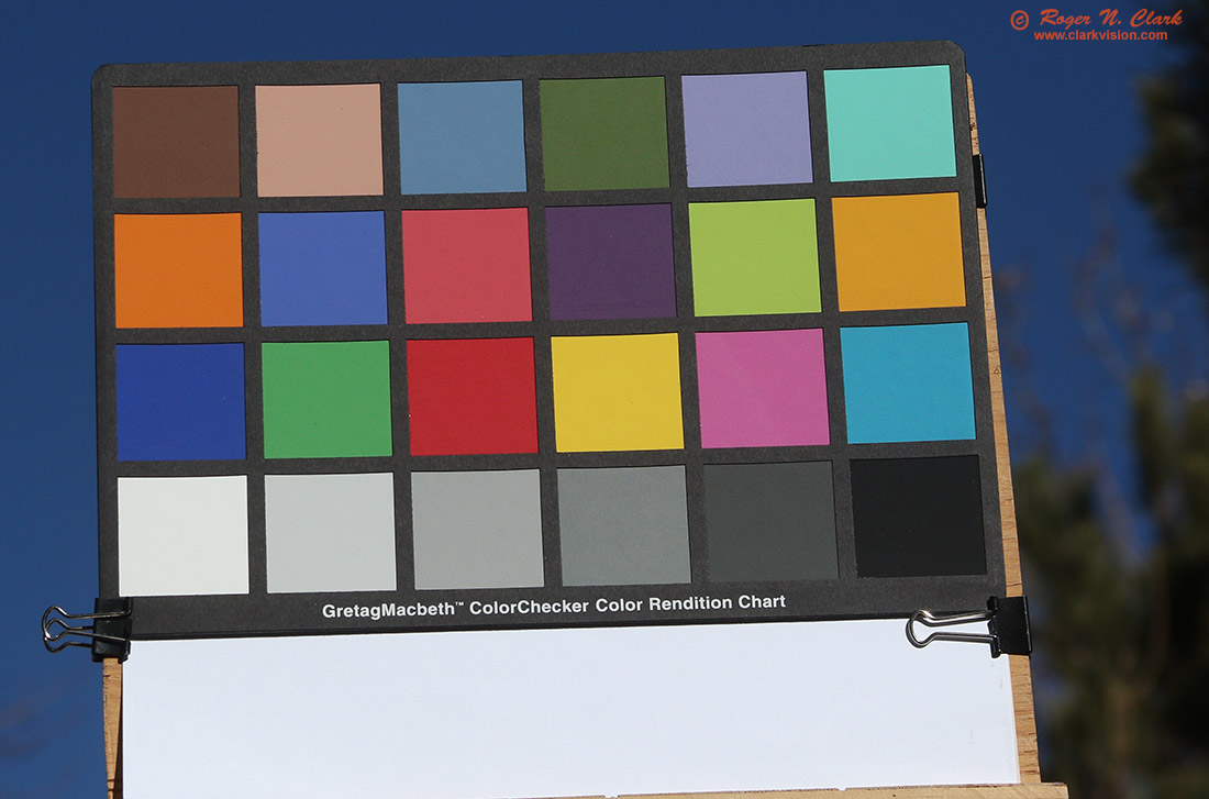
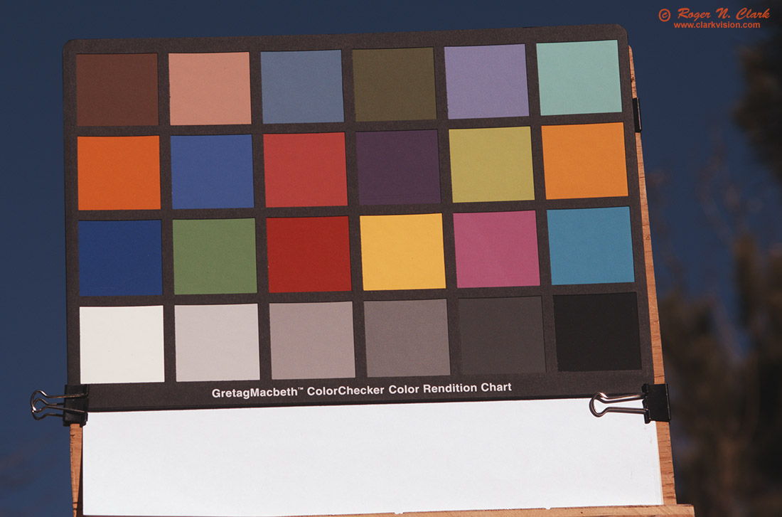
The output of a digital camera color is well calibrated. For example, see Figure 1 where we see a good representation of a MacBeth Color Chart illuminated by the sun from an out-of-camera jpeg.
The typical astro work flow skips critical steps in color production for RGB sensors, whether a color digital camera, or a monochrome camera with RGB color filters. This problem does not apply to narrow band imaging because the images are not intended to be representations of visual color. In the narrow band case, color is used as a representation of the response of a narrow wavelength range, sometimes in the UV or infrared.
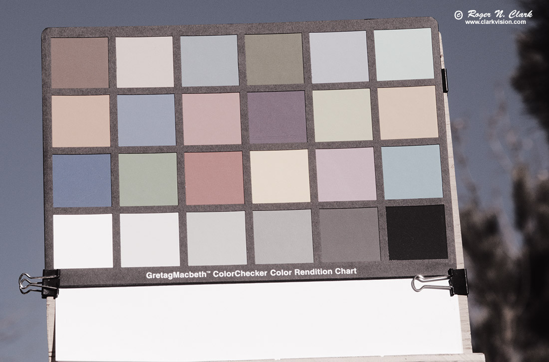
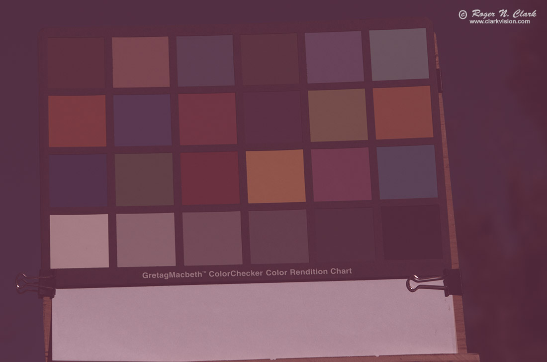
Figures 2, 3, and 4 illustrate the visible RGB color problem. While the examples use DSS, most astro work flow suffers from the same problem. In fact, I only know of one astro software package that included the color calibration steps: ImagesPlus, which, unfortunately is no longer supported.
As illustrated in Figures 2, 3, and 4, the colors are way way off from even being an approximation to reality! This is because the needed calibration steps are not done, including a color matrix correction, tone curve with hue (tint) correction.
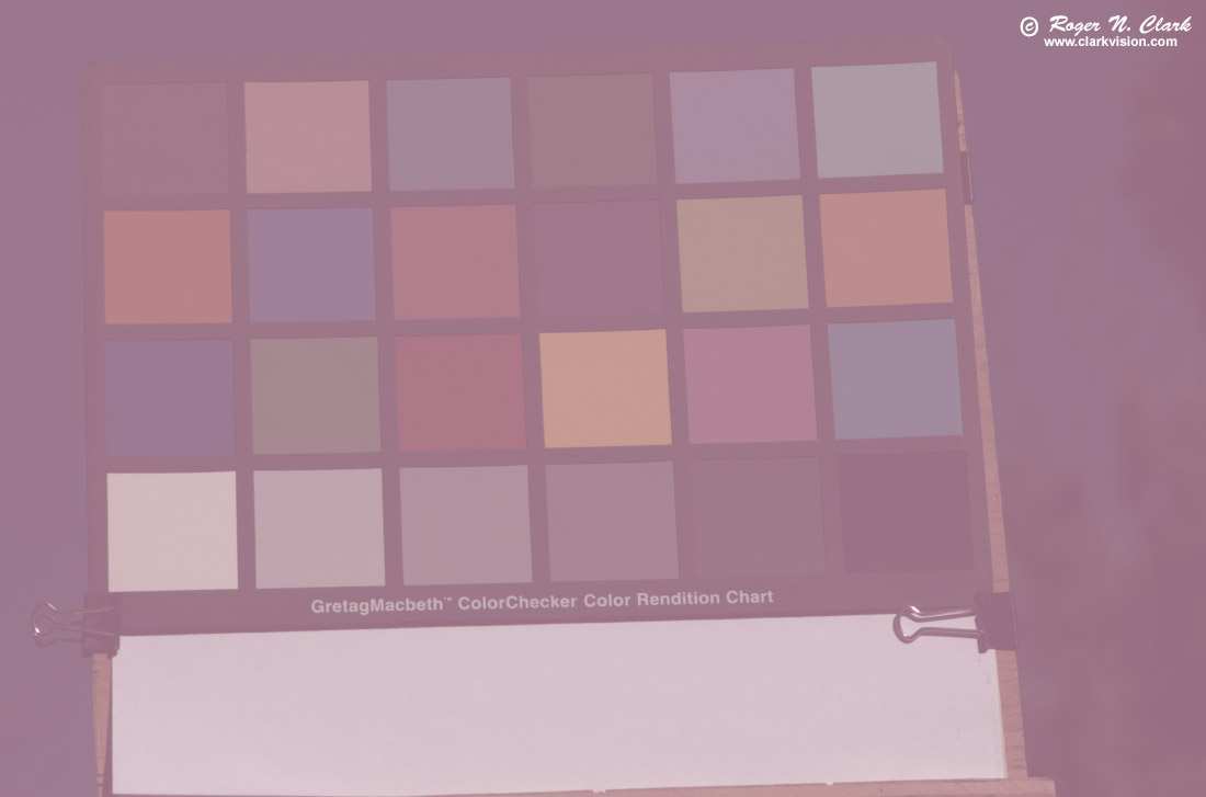
The main reason for poor color out of the astro work flow is the astro work flow does not include needed steps.
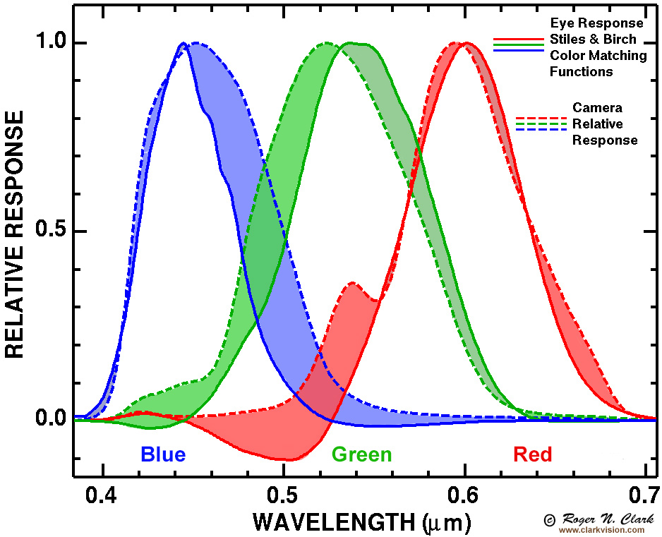
The filters in a Bayer sensor camera are not very good. They have too much response to other colors, so the colors from just straight debayering are muted (e.g. Figures 2, 3, and 4). For example, blue may include too much green and red, red my include too much blue and green, etc (Figure 6). The color matrix correction is an approximation to compensate for that "out-of-band" spectral response problem, and all commercial raw converters and open source ones (e.g. rawtherapee, darktable, ufraw) include the correction. Even the camera does it internally to create a jpeg, including DSLRs, mirrorless cameras and cell phone cameras. Most astro software, however, does not correct for that, so it must be applied by hand.
If you use DSS, pixinsight, or many other astro software packages, the color matrix correction is usually not included, though it can be applied by hand with some software (not DSS), but you have to find the matrix yourself and apply it by hand.
There are two options for finding/making the color matrix if you use dedicated astro cameras. Find a commercial digital camera that uses the same sensor. If DXOMark has reviewed that camera, they publish the matrix, or get a raw file from the camera and use the Adobe DNG converter to create a dng file. The matrix is in the exif data.
The second option is to derive it yourself, e.g. see Color: Determining a Forward Matrix for Your Camera.
The sensor manufacturers should supply the matrix, but unfortunately they do not.
Without the color matrix correction, we see people who use astro software do "color calibration" or "photometric color calibration" but without a color matrix correction that "calibration" is not complete. Photometric color calibration is only a white balance; the color matrix correction is not white balance; it is compensation for out-of-band spectral response. For example, in Figure 3, the white balance is "correct" (e.g. white paper appears white) but the colors are obviously poor. The colors are still muted and sometimes shifted without the color matrix correction, and depending on the nature of this out-of-band response, it can be low saturation and shifted color. Then we see people boosting saturation to try and get some color back, as I did for the image from Figure 4 to get to the image in Figure 5b.
Besides out-of-band color filter response, human color perception is complex. The response is non-linear and response in one color can suppress response in another color. Thus, elaborate models of the human color system have been developed, and these are only approximations. See: Color Part 1: CIE Chromaticity and Perception and Color Part 2: Color Spaces and Color Perception for more information.
Details of the color matrix correction are discussed here:
DSLR Processing - The Missing Matrix.
More details are here:
Color: Determining a Forward Matrix for Your Camera.
The next step in producing an astrophotography image is called stacking. Stacking is averaging images of the same target to reduce random noise and pseudo fixed pattern noise. The term stacking originated from darkroom work where negatives were physically stacked together, aligned and put in an enlarger to make a print with less apparent noise.
Adding images builds signal in proportion to the number of images added, and noise increases by the square root, so S/N improves with the square root of the number of images added. Averaging, what is usually done in stacking, does the same improvement in S/N by square root of the number of images averaged, but in this case, the signal does not increase, and instead the noise floor decreases with the square root of the number of images averaged. Stacking increases dynamic range as well as improving S/N.
The next step, once one has a calibrated and stacked image is to increase brightness of faint objects in the scene. This is called stretching. All our computer monitors and even print media are non-linear, and standards have been developed to compensate for this nonlinearity. The jpeg image out of a digital camera, even a cell phone, or photographic film has a tone curve; a nonlinear response. The image out of a raw converter, e.g. Photoshop, Lightroom, Rawtherapee, etc., has a tone curve applied. But the application of a tone curve shifts color. The hue (tint) correction in a raw converter (and done to make the out-of-camera jpeg) is an approximation to correct for this problem. For more information, see Developing a RAW photo file 'by hand' - Part 2.
Again, the typical astro work flow does not include hue (tint) correction.
In summary, these are the calibration steps need to produce RGB color images.
The typical astro work flow includes manual operations of the above steps 1 - 4, then stacking, then the following.
Photometric color calibration is only accurate AFTER the color correction matrix has been applied to the linear RGB data, the daylight white balance must be applied before the color correction matrix application.
Photometric color calibration, in some implementations, assumes the cores of galaxies are white. It is rare (in fact I know of none). They are typically yellow, like the core of the Milky Way is yellowish-reddish-brown. Assuming white on a yellow target means a shift to blue, suppressing red, contributing to the myth that stock cameras can't record much red hydrogen-alpha emission.
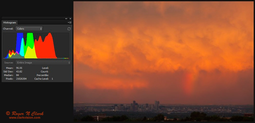
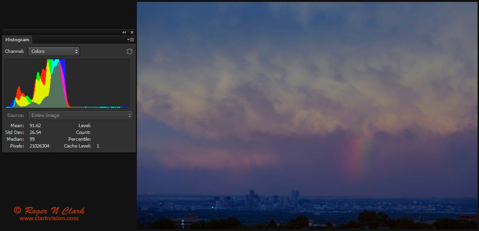
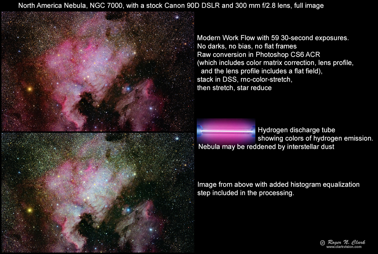
To illustrate how destructive to color calibration a histogram equalization is, examine Figures 7a, 7b and 7c. The histogram equalization step destroyed the red color. Same thing happens in astrophoto processing when a histogram equalization is applied, as seen in Figure 7c.
In the 9 calibration steps listed above, they can all be done automatically with an out-of-camera jpeg, or done completely in a modern raw converter like Rawtherapee, Photoshop, Lightroom, or others. Simply batch convert raw data with these settings, using a modern digital camera, then stack those results. This is what I detail in my Astrophotography Image Processing Basic Work Flow
As noted above, stretching shifts colors. But stretching can also be done with color-preserving stretching software, for example, with the Advanced Image Stretching with the rnc-color-stretch Algorithm which is free, open source.
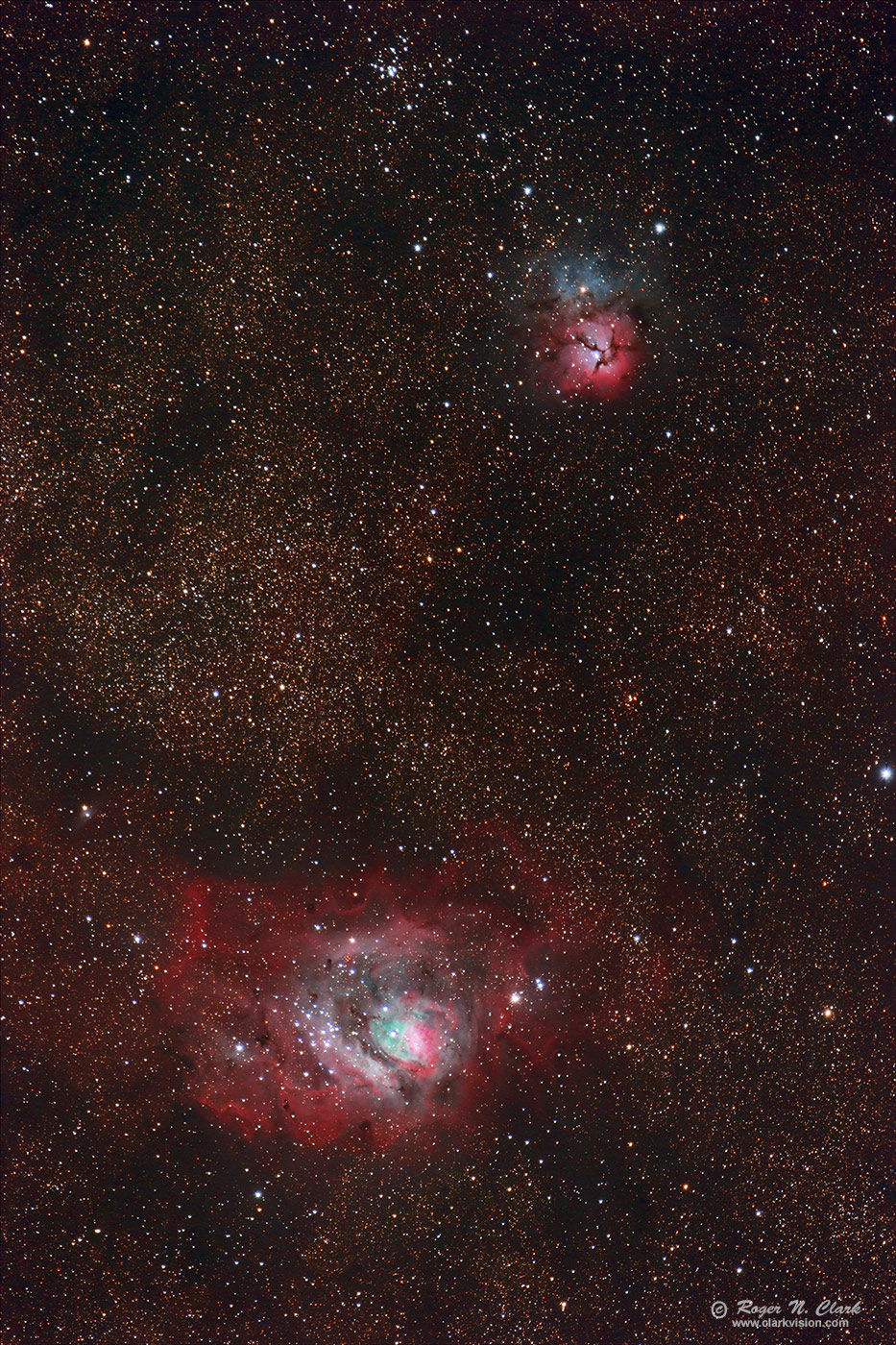
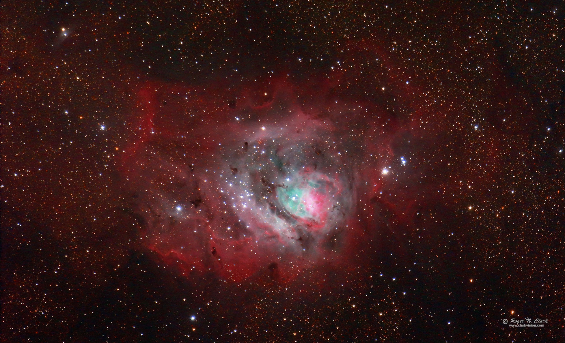
To illustrate how simple this is, see the images in Figure 8a, and 8b, which are produced from out-of-camera jpegs! The image in 8b is an enlargement of M8 from the image in Figure 8a. The image was made by simply stacking out of camera jpegs! To be clear, I don't advocate using jpegs for astrophotography, I only show this to illustrate how well calibrated an out-of-camera jpeg is. How is this possible? Jpeg is 8-bit and raw is typically 14-bit, so there is loss, but the loss is mainly at the high end. The tone curve boosts the low end by a factor of about 40 relative to a 16-bit tiff. The difference between 8 and 14 bit raw data is 4 bits, or a factor of 16. Therefore, the scaling preserves most of the low end at moderate to high ISOs. The main loss is in the high end which gets compressed. See Digital Camera Raw versus Jpeg Conversion Losses for more information on jpeg losses. A single jpeg exposure in the series that produced the image in Figures 8a, 8b adequately digitized the low level noise, and the stacked output was saved as a 16-bit tiff, so the data had plenty of precision. For comparison, here is a single out-of-camera jpeg image with no processing except downsize for web. Note that this image looks far better than a raw file demosaiced to linear in an astro work flow (again look back at Figure 2, 3, and 4). That is because it is very well calibrated.
Figure 9 illustrated the difference in raw data 16-bit processing (rawtherapee and photoshop), versus 8-bit out-of-camera jpegs. The Figure shows similar faint nebula detection of the jpeg processing versus raw processing, but at the high end, stars are bloated in the jpeg result. Rawtherapee shows the smallest stars with more fine detail and similar low level noise.
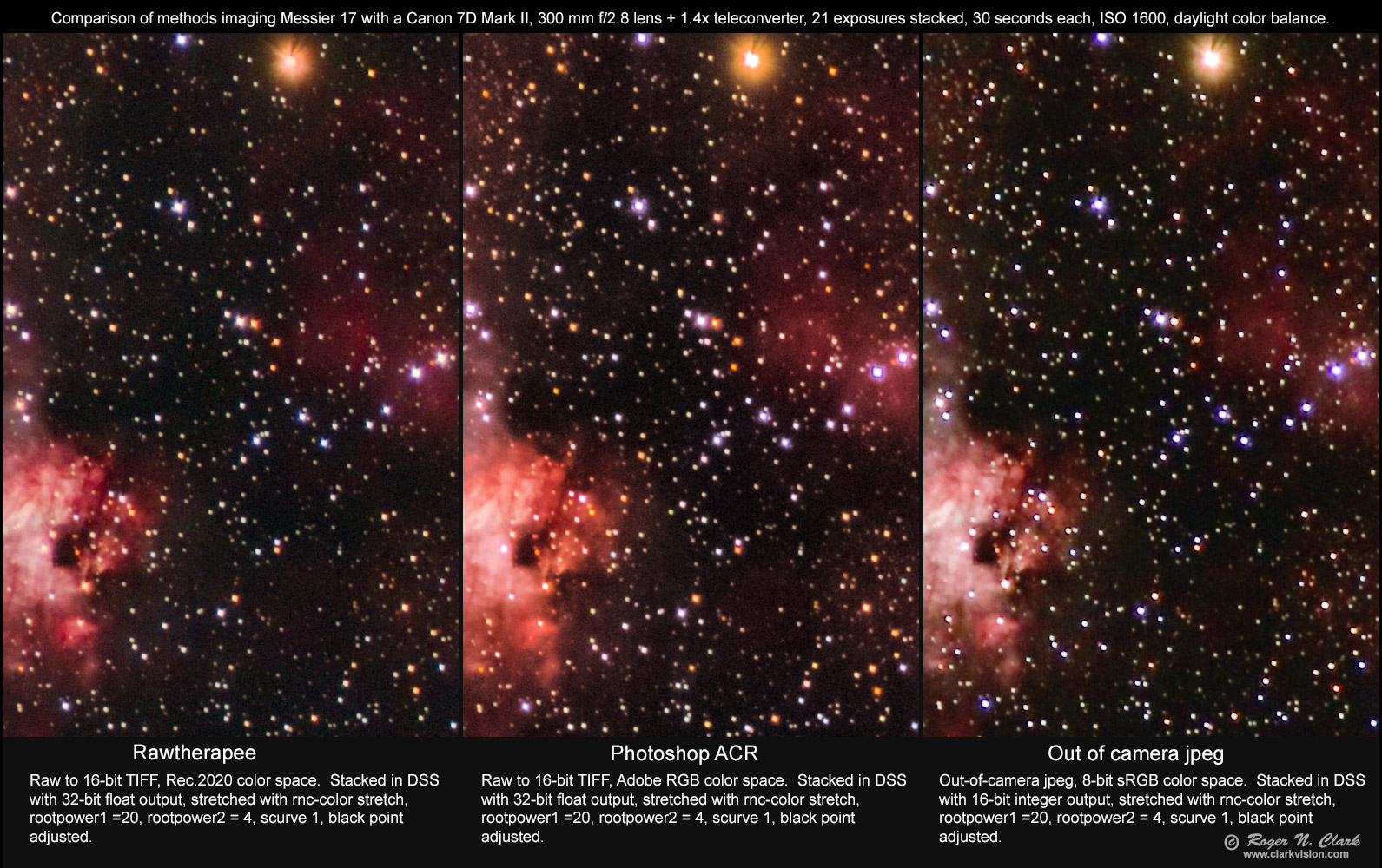
I continue to be amazed by not only the color, but the low apparent noise in images using the modern work flow. This includes out-of-camera jpegs. The internet "knows" that 8-bit jpegs are noisy and contain less data than raw data. However, as early as 2004 I published info that shows that jpeg loss of information is pretty minimal for intermediate to high ISOs. For more information, see Digital Camera Raw versus Jpeg Conversion Losses. That study showed that at mid to high ISOs, there is effectively no loss at the low end, and the main loss is due to the intensity compression from the tone curve at the high end. This is also obvious in Figure 9 where we see similar noise performance at the faint end between raw data processed images and the out-of-camera jpeg, but at the high end, the jpeg saturates the stars at a well before the maximum, resulting in more bloat in bright stars.
To quantify this further, and to compare to a traditional work flow, I calibrated a Canon 90D raw data output values (Data Numbers, DN) and compared the noise performance with Deep Sky Stacker (16-bit output), out-of-camera jpegs (8-bit output), Rawtherapee raw conversion (16-bit output), and Photoshop CS6 ACR (16-bit output; really 15-bits). The results are shown in Figure 10. The results show that the traditional work flow using Deep Sky Stacker, DSS, has S/N lower than out-of-camera jpegs and lower than modern raw converters like CS6 ACR and Rawtherapee. This enables fainter nebulae to be brought out with less exposure time with the use of more modern tools.
The previous sections showed limitations of the traditional work flow, mainly due to the lack of color matrix correction, tint correction, and a common use of color destructive post processing methods, and lower signal-to-noise ratio as seen in Figure 10. But does all this actually impact results?
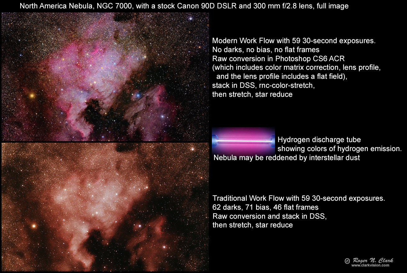
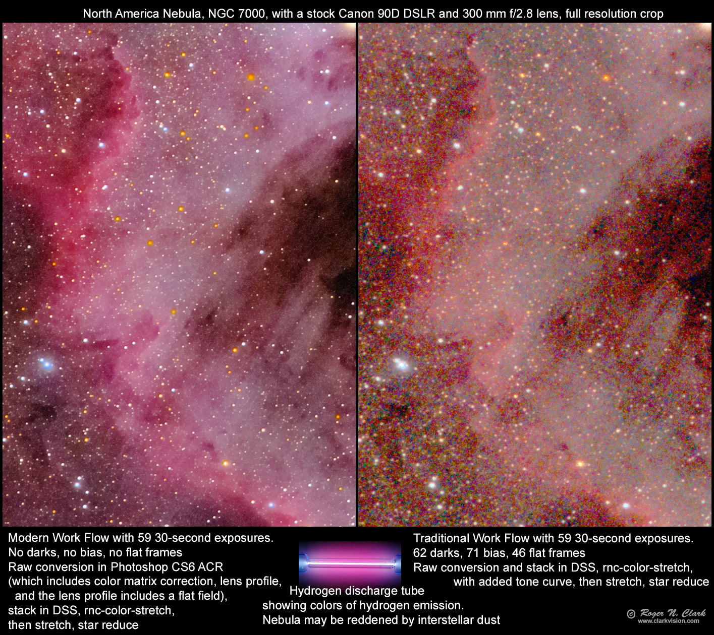
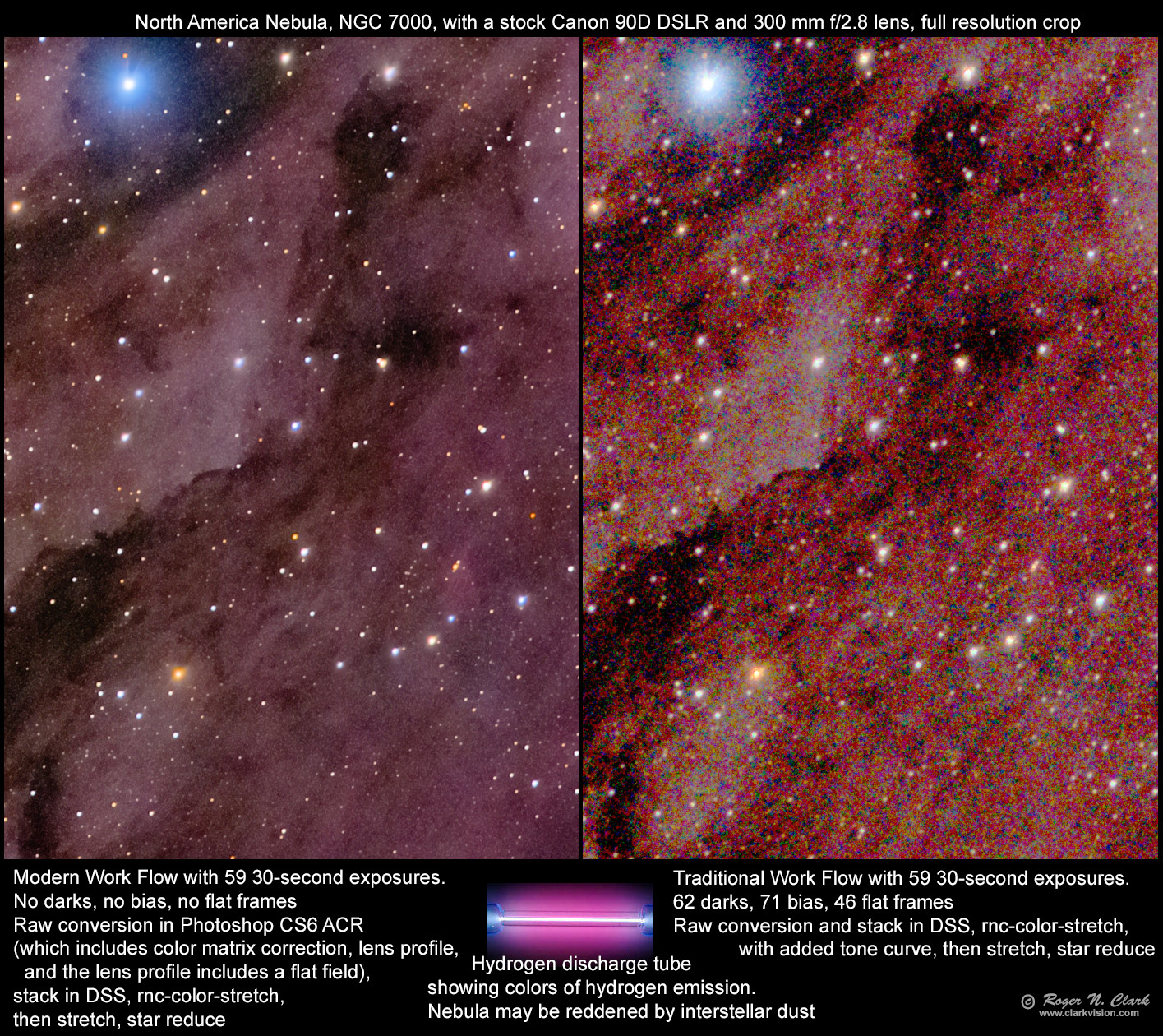
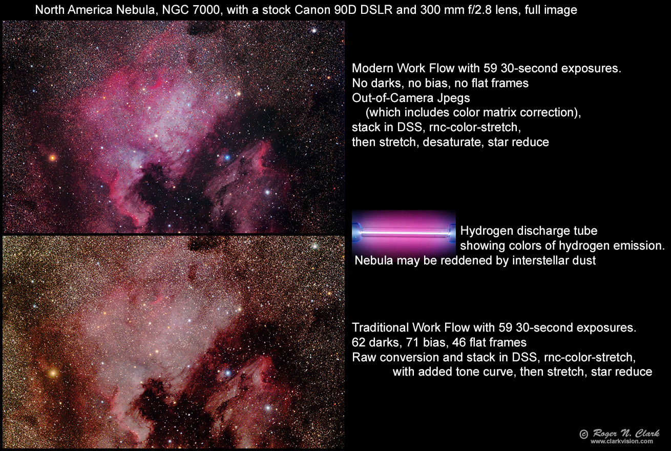
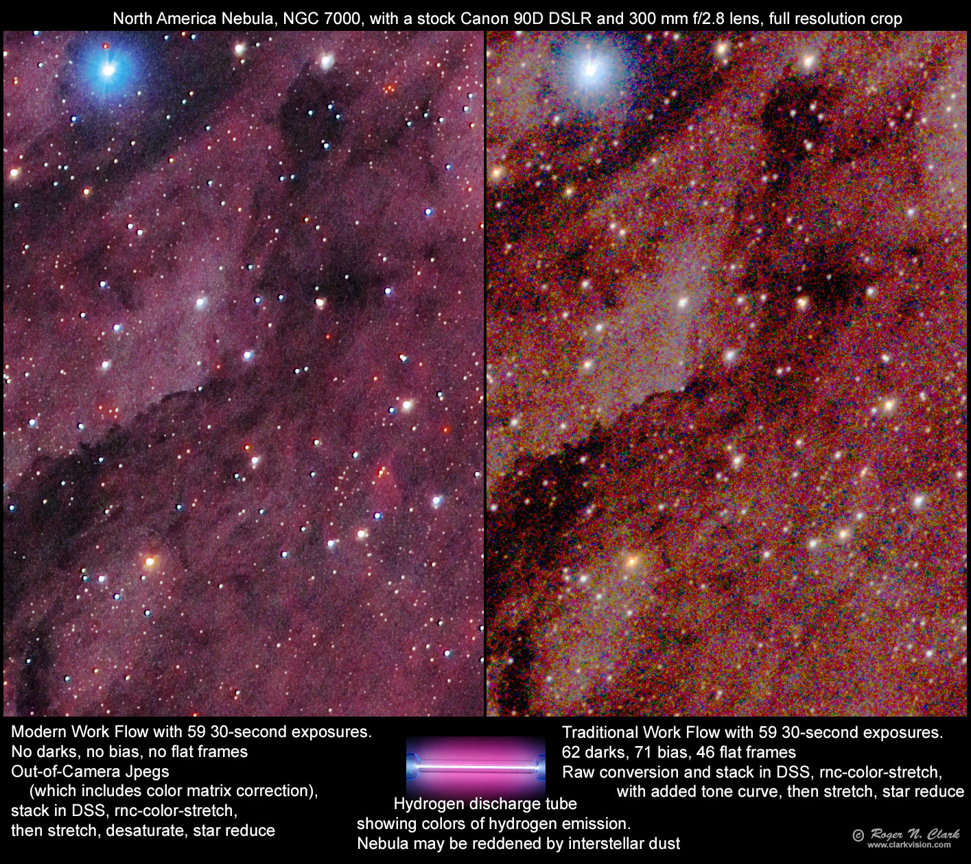
I tested the modern and traditional work flows, and an intermediate method. Using the data that was used to produce this image using a traditional work flow: The North America Nebula and Pelican Nebula gallery image, I tested the traditional work flow with darks, flats, bias frames and tried to equal or surpass the modern work flow result. The modern workflow is described here: Astrophotography Image Processing Basic Work Flow
As shown in equations 2a and 2b, the use of darks, flats and bias frames will increase random noise. Commonly in astrophotography forums, we see that the number of darks bias and flats are typically much smaller than the number of light frames, often 1/3 or less. But to minimize noise from these sources I used more calibration frames than is common. With 51 light frames I made a master dark with 62 dark frames measured at the same exposure time and temperature within 1 degree of the light frames. I measured 46 flat frames and corrected the offset with 71 bias frames. The raw light frames, along with the raw darks, bias and flats were imported to Deep Sky Stacker, DSS, and the lights calibrated and stacked, producing a 32-bit floating point tif file using the same output setting to produce Figure 4, then the linear data were stretched, hopefully to produce color at least as good as seen in Figure 5b. As with Figure 4, the DSS output of NGC 7000 was low in contrast and nearly devoid of color, and being linear data, quite dark.
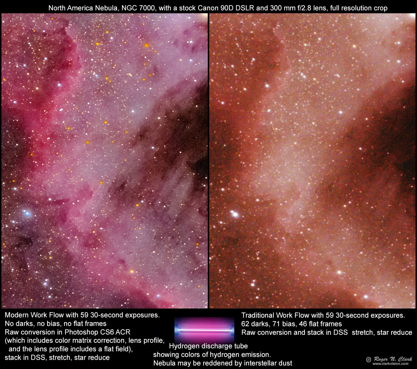
The first effort, is shown in Figure 11a with full resolution crops shown in Figures 11b and 11c. The linear data were stretched with a curves tool using a method to not shift colors significantly (any curves modification changes contrast and saturation in some intensity levels). Brightening with a curves tool compresses the brighter end of the intensity scale lowering saturation, so we see most stars have lost color (what little color they had due to no color matrix correction). The result is a mostly one color image (red-orange to white) (Figures 11a, 11b, 11c). Examining the full resolution crops (Figures 11b, 11c) shows that the image has much greater noise, as expected from the results shown in Figure 10. Also, the stars are larger, despite the fact that the same star size reduction was applied to both traditional and modern work flow results). There is also more color noise in the traditional work flow results.
See if you can use the traditional workflow to make a better image. Here is the DSS stacked image (195 megabytes). All the raw files are here.
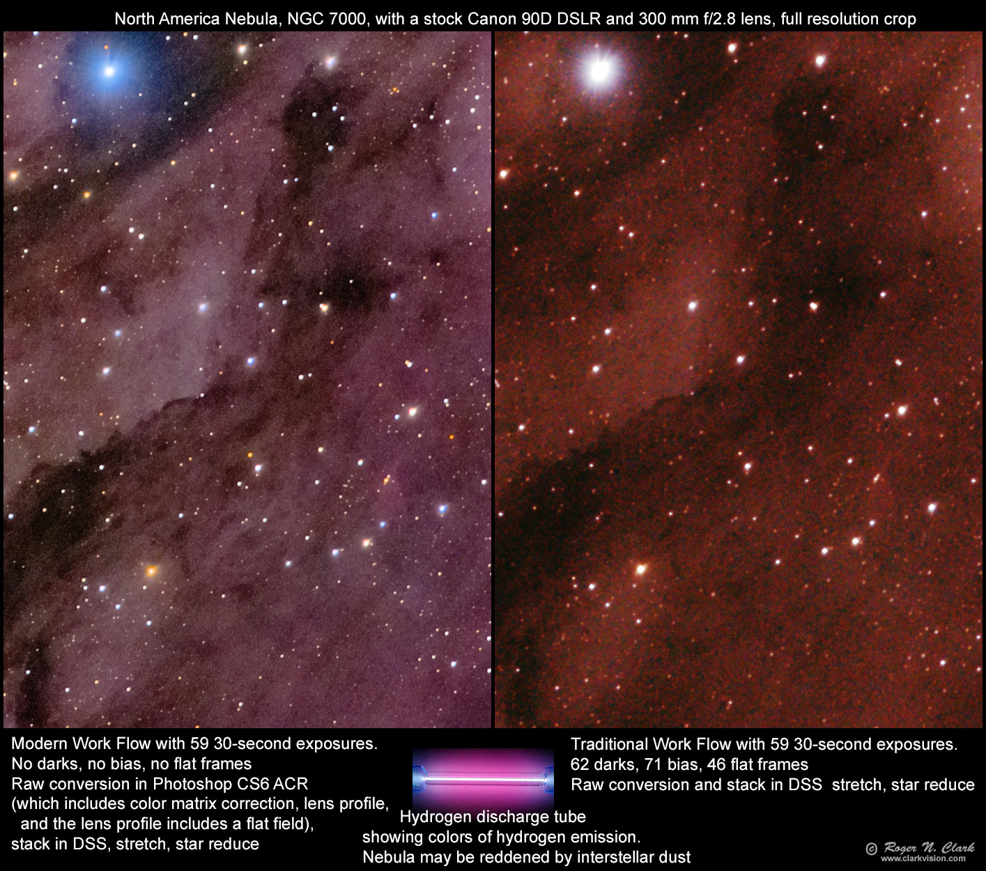
The traditional work flow results seen in Figures 11a - 11c are not very encouraging, so I tried a better method of stretching by including a similar tone curve as the modern work flow followed by a color-preserving stretch with the same parameters as used in the modern work flow. The results, showing better color, are shown in Figures 12a, 12b and 12c. While the colors of the traditional work flow are better, they are still off, but the equal stretch of both modern and traditional work flows shows the huge difference in noise. The traditional work flow shows high noise, and very high chrominance noise. Stars are still larger, and there is less detail. The modern work flow shows significantly lower noise, finer detail and fainter stars.

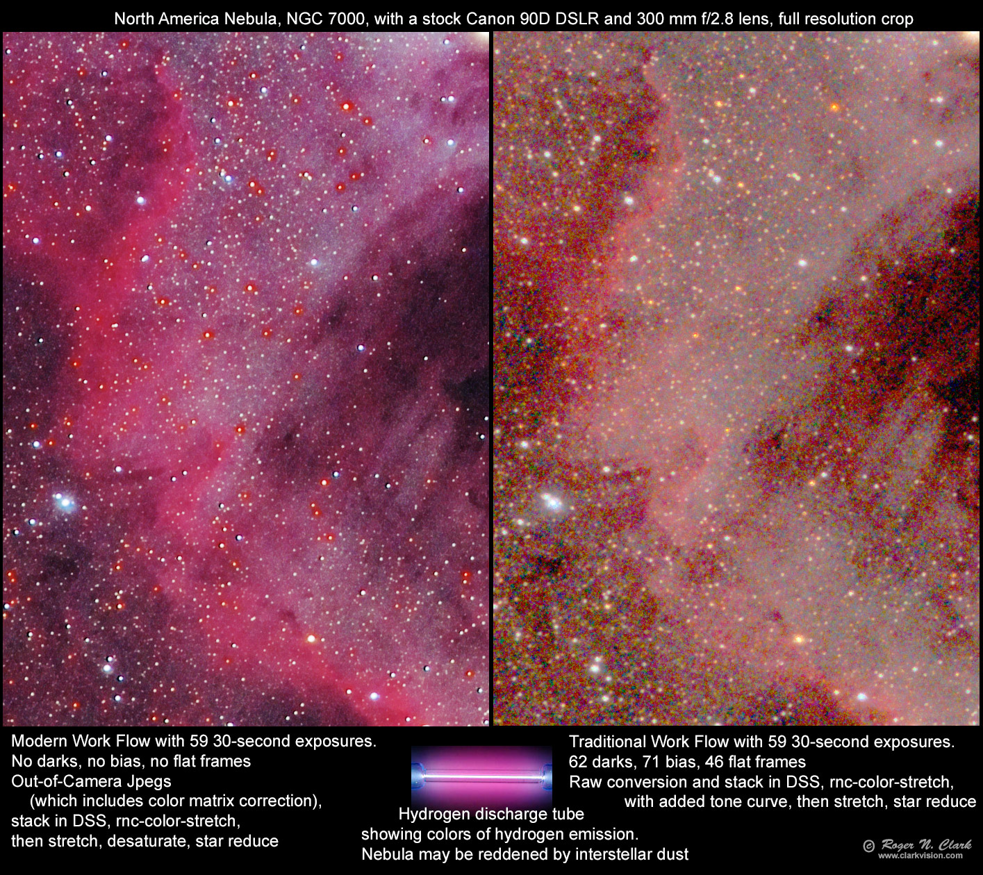
Out-of-Camera Jpegs. The results shown in Figure 10 indicate that out-of-camera jpegs will also have lower noise than a traditional workflow using DSS. This is indeed the case, as shown in Figures 13a, 13b and 13c. The out-of-camera jpegs also show better color and fainter stars. The out-of-camera jpeg rendering algorithm, however, does not do well on red stars, producing a halo (Figures 13b, 13c), but is mostly objectionable when the red stars are superimposed on non-red nebulae. Note this problem was not apparent in the M8 image seen in Figure 8b. The jpegs were the camera default, and changing the in-camera parameters may improve the stars.
Stacking improves signal-to-noise ratio and dynamic range. As discussed in the above section "Simpler Modern Work Flow" and ISOs typically used in astrophotography, the low end is adequately digitized by jpegs and the main loss of information is at the high end of the intensity range. That loss at the high end impacts bright star image quality. Most stars are still smaller than the simple demosaicing algorithm used in DSS 4.2.6 and earlier (as seen in Figures 13b, 13c).
Despite some problems with out-of-camera jpeg star images, an overall better image with lower noise and fainter stars, along with much simpler workflow can be done by stacking out-of-camera jpegs compared to the traditional workflow for making natural color images.
The traditional work flow for processing astrophotos originated in the 1970s, 1980s, and 1990s, and works well for scientific data and single wavelength imaging, but the calibration is incomplete for visible color imaging with RGB sensors found in consumer digital cameras, and in dedicated astro cameras with Bayer color filter arrays (called One-Shot-Color, OSC). The calibration to visible color is also incomplete with the traditional astro work flow using a monochrome camera with RGB filters because no filter set matches the human eye response nor the complexities of human vision.
The same equations to calibrate a sensor from the 1990s are still used today but camera manufacturers have made it simpler by including the equations for calibration inside digital cameras, including in cell phones, DSLRs and mirrorless cameras, both in hardware designs of pixels, and in software (firmware to produce in camera jpegs, and in raw converters to process raw files from a camera).
Production of calibrated color from a digital camera has never before been as simple if modern work flow is adopted. The traditional astro work flow skips critical steps in color production, leaving photographers who use astro-processing software struggling with color.
Using modern tools, like rawtherapee, photoshop, lightroom and others, color production and accuracy is made much simpler and can result in images with lower noise. Even out-of-camera jpegs can have better signal-to-noise ratio than seen in a traditional work flow! See: Astrophotography Image Processing Basic Work Flow
The bottom line is that with modern digital cameras (DSLR or mirrorless) calibration of any photo, daytime or astro is very simple, including no need to make bias or dark measurements. In better modern cameras, the fixed pattern noise is so low that not including darks and bias frames can produce a better image. That still means calibration with bias value (single number), and flat fields. Flat field correction is included in modern raw converters in lens profiles, for those using lenses.
The traditional work flow does not include a color matrix correction and with the measured calibration frames, each with random noise, results in images with low color fidelity and higher noise. Some astro programs use simple demosaicing algorithms and produce lower resolution images with higher noise, especially higher chrominance noise.
If you do the "astrophotography" manual work flow, test that work flow on everyday images, including outdoor scenes on a sunny day, red sunrises and sunsets and outdoor portraits. How good are the results, even compared to an out-of-camera jpeg? You'll likely find that if you use the astrophoto software and traditional lights, darks, bias, flats work flow, it won't be very good, and that is because important steps are missing. And if you are doing wide field imaging, flat fields are very difficult to get right. To be clear, the astrophotography software is capable of including the missing steps, but it is rare to find them in online tutorials, and it is up to the user to actually use them, but including all the steps is complex.
Here are examples: all images in the last ~dozen+ years were made with stock, unmodified, uncooled DSLRs and mirrorless cameras with no bias frames, no dark frames and no measurement of flat fields and a modern work flow: my astrophoto gallery.
If you use older cameras, or dedicated astro cameras, you will need to do the traditional work flow, but include the missing steps, like color matrix correction if you want good color.
If you use digital cameras but a telescope instead of a stock lens, there will not be a lens profile. You will need to measure your own flat field. Rawtherapee can include a flat field, or you can use Adobe's lens profile creator to create a custom lens profile for your telescope. If you use rawtherapee and feed it a flat field, it must be a single raw file. You can make a "master flat" using many exposures then use a tool to convert that master flat to a raw DNG file. Rawtherapee can use that dng file.
Digital cameras continue to improve even over the last few years. Key improvements include better Quantum Efficiency (QE), lower noise floor, lower dark current, better low signal uniformity, and lower pattern noise.
Avoid cameras that filter raw data. Variations in filtered raw data vary from deleting stars to turning star color to green or magenta (there are no green or magenta stars). For a partial list of camera models known to filter raw data see the links in this page: Image Quality and Filtered Raw Data
Large vs small pixels. Online one often sees the myth that larger pixels are more sensitive. However, adding signal from multiple small pixels to form a larger pixel gives about the same total signal as a large pixel of the same area. Cameras with large pixels tend to show more pattern noise, e.g. banding. Higher megapixel cameras, especially recent models, which have smaller pixels, tend to have less pattern noise and better low end uniformity.
Choose models that have a self-cleaning sensor unit (ultrasonic vibration of the filters over the sensor). Set up the camera to automatically clean the sensor when it is turned on or off. Run the cleaning process before a long imaging session. Minimize the time the camera is exposed with no lens or body cap on. For example: Minimize Dust Contamination.
Choose the most recent camera you can afford for better low level uniformity and better on-sensor dark current suppression technology. Camera models from the last 2 or 3 years show significant improvements over earlier models and have better low light uniformity, low dark current, excellent dark current suppression technology and more models with flip-out screens to better dissipate heat. Mirrorless and DSLR models that do high rate 4K video may also have improved heat dissipation. Bottom line is to buy the most recent camera models you can afford. Many are excellent for astrophotography as well as regular daytime photography, and sports and wildlife photography. More info at: Characteristics of Best Digital Cameras and Lenses for Nightscape, Astro, and Low Light Photography Note: this is not a list of specific models, but what to look for in a camera.
NASA APOD: Dark Dust and Colorful Clouds near Antares This is the best image of this area that I have ever seen.
NASA APOD: Spiral Meteor through the Heart Nebula
NASA APOD: Eclipsed Moon in the Morning
M45 - Pleiades and surrounding dust from very dark skies
The Sadr Region of the Milky Way with a cheap barn door tracker I made
M31 - Andromeda Galaxy [20mins exposure]
Veil Nebula from bortle 2 skies with unmodded DSLR
The Witch Head nebula looking at Rigel
The Pleiades (M45) - The Seven Sisters
If you have an interesting astro image processed using my modern methods, please let me know and I'll consider including a link here.
References and Further Reading
Clarkvision.com Astrophoto Gallery.
Clarkvision.com Nightscapes Gallery.
Goossens, B., H. Luong, J. Aelterman, A. Pizurica and W. Philips, 2015, An Overview of State-of-the-Art Denoising and Demosaicing Techniques: Toward a Unified Framework for Handling Artifacts During Image Reconstruction, 2015 International Image Sensor Workshop. Goossens.pdf.
The Night Photography Series:
| Home | Galleries | Articles | Reviews | Best Gear | Science | New | About | Contact |
http://clarkvision.com/articles/sensor-calibration-and-color/
First Published July 6, 2022
Last updated January 5, 2024