ClarkVision.com
| Home | Galleries | Articles | Reviews | Best Gear | Science | New | About | Contact |
Image Processing: Stacking Methods Compared
by Roger N. Clark
| Home | Galleries | Articles | Reviews | Best Gear | Science | New | About | Contact |
by Roger N. Clark
Image Stacking improves signal-to-noise ratio, but not all stacking methods are as effective. This article shows some differences and which ones are best and the data format to use.
The Night Photography Series:
Contents
Introduction
The Test Data
Results
Real-World Image Example
Sampling in the Camera
Conclusions
References and Further Reading
Questions and Answers
Many terms we have today in photography originated with darkroom techniques (like dodge and burn). Stacking is another such term. Stacking refers to physically stacking negatives, aligning them and then putting the stack in an enlarger to make a print. It is tedious and difficult. Stacking averages film grain. With digital photography stacking is aligning a group of images digitally and averaging them (or compute the median, but average is better). There are free as well as commercial tools to do stacking.
Stacking is a term for adding/averaging multiple images together to reduce apparent noise (improve the signal-to-noise ratio) of the combined image. The signal-to-noise ratio, or S/N, increases by the square root of the number of images in the stack if there are no side effects. But in practice, there are side effects, and those side effects can result in visible problems in stacked images and limit the information that can be extracted. Which method(s) work best with the least artifacts?
There are basically 2 methods:
1) a form of add/average, including graded averages, sigma clipped average, min/max excluded average, etc.
2) median including clipped median, min/max exclusion, etc.
The effectiveness of stacking depends on the data that are fed to the stacking software. The raw output of most digital cameras is 14 bits per pixel. A raw converter may create the following:
a) linear 14-bit data from the DSLR, unscaled,
b) linear 16-bit data scaled by 4x from the 14-bit DSLR data, and
c) Tone curve 16-bit data.
To investigate the effectiveness of two different stacking methods, a standard deviation clipped average (called Sigma Clipped Average), and Median calculation, stacking was tested using different data types: linear 14-bit, linear 16-bit, and tone mapped 16-bit data.
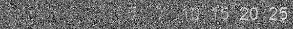
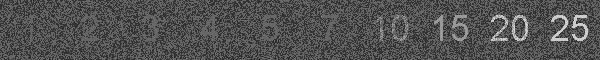
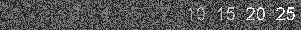
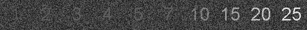
To test the effectiveness of stacking, I constructed an image with embedded numbers (Figure 1). Then I scaled the numbers into an intensity sequence (Figure 2). Using scientific image processing software (Davinci from Arizona State University, http://davinci.asu.edu/), I computed images of random Gaussian noise. To the image in Figure 2, I added an offset, typical of Canon DSLRs to keep signal and noise from clipping at zero in the integer image files. I computed random noise at a level that made the S/N = 1.0 on the number 10 in the image. That means the number 1 has a S/N = 0.1 and 25 has S/N = 2.5 in a single image file. An example single image with noise is shown in Figure 3.
One hundred images like that in Figure 3, each with different random noise, were computed for stacking tests. The first set of 100 images simulates the output of a DSLR with 14-bits per pixel. A second set of 100 was computed as from a DSLR with linear 14-bits per pixel, then scaled by 4x to scale the 14-bits to 16 bits like that from some raw converters. A third set of 100 images was computed and scaled as if in a tone curve output from a raw converter. Because the test is for the faintest parts of an image, the tone curve scales the data by a factor of 10 but the response is still linear (see part 3b for more information on the tone curve function). The 16-bit data and tone curve data are still quantized at 14 bits but the scaling potentially adds precision to the stack, and we will see the effects of what the scaling has on the final output.
Stacking was performed in ImagesPlus selecting two methods: median and sigma clipped average. The clipping was set to 2.45 standard deviations. Clipping in a real image stack of the night sky removes most signatures from passing airplanes and satellites. In the data test here, there is essentially no difference in an simple average versus a clipped average.


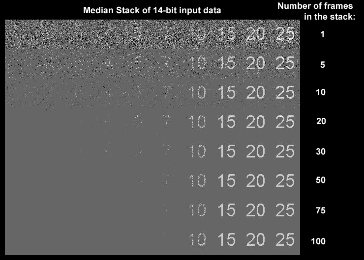
The results of the 14-bit linear output are shown for a median stack in Figure 4a and a Sigma Clipped Average stack in Figure 4b. The clipping was set to 2.45 standard deviations. Clearly, the Sigma Clipped Average produces a better result. The median is posterized to 14 bits, and it would be impossible to pull out faint signals But even the 14-bit linear data are posterized and limited information could be extracted (the numbers below 10).

The results of the 16-bit linear output are shown for a median stack in Figure 5a and a Sigma Clipped Average stack in Figure 5b. The clipping was set to 2.45 standard deviations. Again, the Sigma Clipped Average produces a better result. The median is quantized to 14 bits. The median stack shows the numbers less than 10, but each number has a constant intensity level and the background has another constant intensity level. The Sigma Clipped Average produces a smoother result with decreasing intensities on the numbers, as expected, and a lower noise background. The Sigma Clipped Average also shows better separation of the numbers from the background. This means that fainter stars, nebulae and galaxies can be detected in an astrophoto.
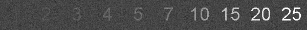
The results of the tone curve output are shown for a median stack in Figure 6a and a Sigma Clipped Average stack in Figure 6b. The clipping was set to 2.45 standard deviations. Again, the Sigma Clipped Average produces a better result. The median is quantized to 14 bits and appears similar to that in Figure 5a, but slightly less noisy. The median stack shows the numbers less than 10, but each number has a constant intensity level and the background has s slightly different constant intensity level. The Sigma Clipped Average produces a smoother result with decreasing intensities on the numbers and a lower noise background. The noise in the Sigma Clipped Average result (Figure 6b) is lower than that in the 16-bit linear stack (Figure 5b).

In Figure 7, I compare the three methods for the median stack. Of these three, the tone curve results are the best, but all the median results are inferior to the Sigma Clipped Average results.
In Figure 8, I compare the three methods for the Sigma Clipped Average stack along with a full 32-bit floating point stack. Of the first three, the tone curve results are the best and visually indistinguishable from the 32-bit floating point results.

To detect the smallest signals in a stacked exposure set, sampling in the camera should be high enough to digitize those tiny signals. Figure 10 shows sampling effects by the camera A/D in a low noise situation (low camera noise).
It shows that to detect photons at the sub photon per exposure rate, there is an advantage in going higher than unity gain (higher ISO) (higher gain is smaller e/DN). (DN = data number in the image file). In night sky photography, as noise from sky glow increases, the benefits are reduced. One also sees from the diagram that there is not much gain in faint object detection by going from 0.3 to 0.2 e/DN (that would be a 50% increase in ISO), but a fair jump in faintest details digitized in going from unity gain to 1/3 e/DN. The image data are normalized so that the number 25 appears the same brightness.
In the 100 image stack, by digitizing at 0.3 e/DN, 20 photons are just detectable, or a rate of 1 photon per 5 images on average. At unity gain it is about 4 times worse. In real-world cameras with some banding present, the differences between gains will be larger. This implies over a stellar magnitude detection difference in astrophotography.
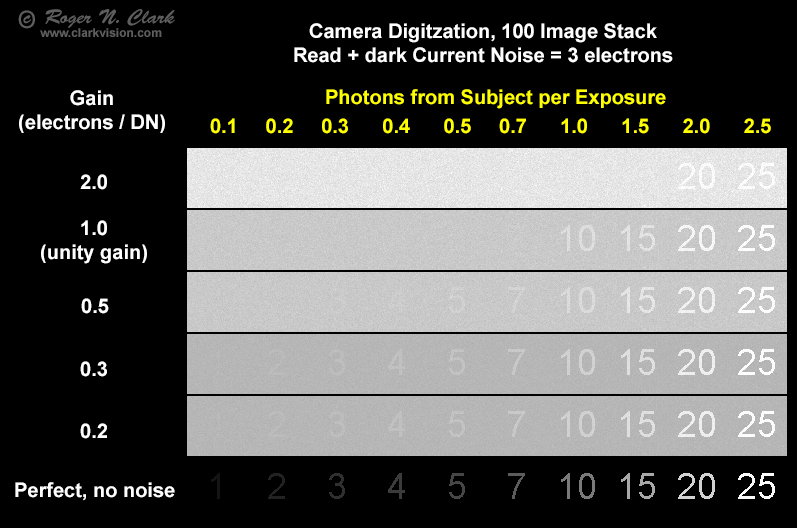
The model used to make the data in Figure 10 used a Poisson distribution for the photon noise, Gaussian distribution for the read + dark current noise, and +/- 1 DN error in the A/D conversion, then scaled the output images to the same level for comparison. The A/D error is important. For example, say you had 1 photon in a pixel in each exposure, the A/D will have some with no photons, and some with 2, thus increasing the error. Of course the other noise sources modulate that, but including the A/D conversion noise is important in showing the trend. As other noise sources increase, the A/D effect becomes less and it is less important to work at higher ISOs, unless one also needs to overcome banding problems (which is often the case).
The key to astrophotography in detecting faintest details are:
1) Darkest skies you can get to.
2) Largest aperture quality lens/telescope you can afford, with fastest f/ratio. Fast f/ratio and large aperture are key because you gather the most light in the shortest time.
Camera operation: ISO where a) ISO where banding in small enough to not be a factor, b) gain (ISO) about 1/3 e/DN. If banding is still an issue at ISO 1/3 e/DN, then go to higher ISO.
In choosing a digital camera for astrophotography:
1) Recent models from the last couple of years (these models, all manufacturers) have better dark current suppression and lower banding as well as good quantum efficiency.
2) Lowest dark current.
3) Models with no raw lossy compression or raw star eating filtering and minimal raw filtering (at least 2, maybe more manufacturers are great in this area).
If read noise is on the order of about 2 or 3 electrons (or less) at ISO gain of 1/3 e/DN and low banding at that DN, having lower read noise will not show any difference in long exposure astrophotography where you can record some sky glow in each exposure. Only if you are trying to do astrophotography with couple of second exposures with narrow-band filters or very slow lenses/telescopes would read noise become an issue.
Where a camera becomes "ISOless" is largely irrelevant in astrophotography because ISOless is about low read noise and read noise gets swamped by other noise sources. Again, it is good to have reasonably low read noise (meaning 2 to 3 or so) at an ISO gain of about 1/3 e/DN. Sure it is fine to have lower, but it makes little difference when you expose sky to 1/4 to 1/3 histogram, then add in noise from dark current. These noise sources are what limit dynamic range and faintest subject detections, NOT read noise and whether or not you are at an ISOless level or unity gain.
Bit precision and method are important in stacking. The averaging methods are superior to median combine. As digital cameras get better, with lower system noise, including read noise and noise from dark current, and as more images are stacked, the output precision of the stack must be able to handle the increase in the signal-to-noise ratio. Simple 14-bit precision is inadequate, as is 14-bits scaled to 16-bits (only a 4x improvement in precision) when stacking more than about 10 images. When stacking large numbers of images, the increase in precision can only be met using averaging in 32-bit integer, 32-bit floating point or tone mapped if 16-bit image files are used.
If you are working with large numbers of images in a stack and want to work in a linear intensity response, then it is best to use an image editor that can work in 32-bit floating point, including storing the stacked image in a 32-bit integer or floating point format.
Tone mapping gives an approximately 40x improvement in intensity precision for the faintest parts of an image when working with 16-bit files compared to linear 14-bit digital camera raw output. Thus, tone mapping allows one to extract fainter details when working with 16-bits/channel image editors and 16-bits/channel format image files. If we assume a 1-bit pad in precision, the 40x scaling of the faintest tone mapped data would be good for 20x improvement in S/N, which means stacking up to 20 squared or 400 images should still work with adequate precision.
Of course, encountering these effects also depends on the noise levels in your imaging situation, including noise from the camera system and noise from airglow and light pollution. As noise increases, these side effects become hidden (literally lost in the noise).
If stacked images are done in linear 14 or 16-bit output, you may run into posterization, which shows as "splotchiness" and what I call a pasty look in images when stretched. I see a lot of these artifacts in online posted astrophotos, which indicates to me that posterization in the stacking is likely occurring.
The trade point of when a float is needed depends on the noise level (including read noise plus noise from dark current and noise from airglow and light pollution). One way to check this is to do some statistics on a single exposure in a dark area with no stars or nebulae. Let's say you do that and find a standard deviation of 6.5. If you then stack more than 6.5*6.5 = 42 frames, then the result will be integer quantized and extracting the faintest detail will be limited by integer math. Then it would be better to save the result of the stack as a 32-bit float format and stretch the results from the 32-bit float data. In ImagesPlus, you can keep the default format at 16-bit, and then at the end of the stack, save a copy of the image, select fits, then select 32-bit float format.
Why is the median stack image in Figure 4a flat with a single value for the background?
Answer. When the input data are quantized, the median combine is also quantized. Even if the input data are scaled to floating point values, they are still quantized (e.g. multiply by 1.23 and carried as floating point, there are still discrete values just now separated by 1.23). The median combine chooses one of those quantized values as the median. By stacking many images, when the noise in the stack is reduced to a fraction of the quantization step, the median gets quantized to a single value. Technically, this occurs when the standard deviation of the median is less than the quantization interval, and becomes significantly posterized when the standard deviation of the median is about 1/4 the quantization interval. How many images need to be combined for this to happen with real data depends on the quantization interval and system noise. But once posterization starts, adding more frames accelerates the collapse (Figure 11) and one can not extract a fainter signal from the data. Again, it illustrates that a median combine should be avoided when stacking image data.
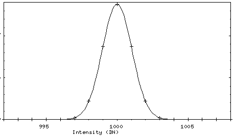
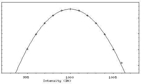
The next question is, is the generated noise really Gaussian? Figure 12 shows linear and log plots of the noise profile (crosses) and Gaussian profile (line). The data are Gaussian within counting statistics (+/- 1). The online posts have charged the data are not Gaussian, but confuses Gaussian profile with sampling interval.
On why the median combine in Figure 9a is noisier:
"Also, specifically for light, photons tend to arrive in bundles or waves,
sometimes causing a disruption in the expected Poisson distribution. And
that's something that should not be ignored. The result of these clumps
of extra photons or periods of no photons is a possible disruption the
median value, moving it higher or lower than it should have been. I
think this not only leads to nosier result than an average, but also
less quantization exactly *because* there is *more* noise. Again, your
Figure 9 median combine with real data shows this. There is a nosier
median than the average, as expected from statistical mathematics."
Answer. First, the input data (raw files) are exactly the same for all methods in Figure 9. If noise from photon clumping were a factor then we would see that the same pixels in the images made with other methods to also appear noisier. We do not. Second, see The Present Status of the Quantum Theory of Light edited by Jeffers, Roy, Vigier, and Hunter, Springer Science, 1997, page 25, where the clumping is described as being observed from astronomical objects on a few meter scale. At the speed of light, that applies to a few nanosecond scale, compared to the 4260 second exposure time of the Horsehead image in question. The photon clumping idea is off by some 12 orders of magnitude. The data in figure 9a is purely a consequence of median quantization.
On why noise is different between the images "Noise is worse than 25% because you did multiple operations, each adding its own error. Applying darks and flats also add noise. The 80% S/N is just for 1 simple median. Honestly, if you didn't realize that there should be extra error that then I don't know what to say."
Answer. All image combine stacks were performed in ImagesPlus which used 32-bit floating point. The input data from a DSLR of course are quantized and remain so after conversion to 32-bit floating point. The 32-bit floating point calculations ensure that there is no significant error added by the stacking operations. Also, the exact same master dark frame, flat field and bias frames were used for both the median and the average, so if the errors were due to these data, it would show in both the median and average stacks. Obviously it does not.
References and Further Reading
Clarkvision.com Astrophoto Gallery.
Clarkvision.com Nightscapes Gallery.
The open source community is pretty active in the lens profile area. See:
Lensfun lens profiles: http://lensfun.sourceforge.net/ All users can supply data.
Adobe released a lens profile creator: http://www.adobe.com/support/downloads/detail.jsp?ftpID=5490
More discussions about lens profiles: http://photo.stackexchange.com/questions/2229/is-the-format-for-the-distortion-and-chromatic-aberration-correction-of-%C2%B54-3-len
Tech Note: Combining Images Using Integer and Real Type Pixels. This site also shows median combine not producing results as good as mean methods: http://www.mirametrics.com/tech_note_intreal_combining.htm.
Notes:
DN is "Data Number." That is the number in the file for each pixel. It is a number from 0 to 255 in an 8-bit image file, 0 to 65535 in a 16-bit unsigned integer tif file.
16-bit signed integer: -32768 to +32767
16-bit unsigned integer: 0 to 65535
Photoshop uses signed integers, but the 16-bit tiff is unsigned integer (correctly read by ImagesPlus).
The Night Photography Series:
| Home | Galleries | Articles | Reviews | Best Gear | Science | New | About | Contact |
http://clarkvision.com/articles/astrophotography.image.processing
First Published July 8, 2015
Last updated January 15, 2022