ClarkVision.com
| Home | Galleries | Articles | Reviews | Best Gear | Science | New | About | Contact |
Night and Low Light Photography with Digital Cameras (Technical)
by Roger N. Clark
| Home | Galleries | Articles | Reviews | Best Gear | Science | New | About | Contact |
by Roger N. Clark
The Night Photography Series:
Contents
Introduction
Night photography of City Scenes
Low Light with Moving Subjects
Long Exposure Deep Sky Low Light Imaging
Very Low Light Imaging
Light Intensities Under Different Lighting Conditions
A Moonlit Scene
Astronomical Imaging
Discussion
Improving Photon Collection
Other Digital Cameras
References
Introduction
Night and low light photography places some very demanding constraints on photography. Compared to daytime photography, night and low-light photography in the digital age hits new limits, including noise due to photon statistics, read noise from digital sensors, with limits imposed by transmission of optics and the quantum efficiency of detectors.
The phrase "low light" is key. Light is finite. One can't magically turn up sensitivity and see more light and more detail in a scene. The light, or number of photons is low. The noise we see on most digital camera images is mostly due to that from photon noise: the random arrival of photons over our exposure time. The noise is the square root of the number of photons collected during the exposure.
Increasing ISO on a digital camera does not change the sensitivity of a digital camera, contrary to what you may read in reviews, photo magazines and books, and even manufacturers specifications. Digital cameras have one sensitivity set by the quantum efficiency of the sensor. Changing ISO simply changes an electronic gain after the sensor to boost the tiny electronic signals from the sensor, and instructs the camera to meter for a shorter exposure time or slower f/ratio. The sensor in digital cameras have analog-to-digital conversion circuits with less dynamic range than the sensor. At low ISO, signals from low light on the sensor get swamped by post sensor electronics. Boosting ISO changes the post sensor gain so one sees the lower signals from the sensor. Future cameras will likely have better analog-to-digital converters so this is no longer a problem and ISO could be a post processing option.
The bottom line in Low light means the number of photons per second is low, so one has to compromise and expose longer if you want a low noise image (high signal-to-noise ratio), versus accept noise if you must keep exposure times short to reduce subject blur. Implications of these basic physical facts will be discussed below in the section on improving light collection.
As noted above, ISO does not change sensitivity. Low ISO instructs the electronics to digital more of the full range capability of the sensor. An analogy to collecting light with a pixel is like collecting water in a liquid measuring cup. Low ISO uses the full cup to measure how much liquid is in the cup. Double the ISO and you measure up to half the cup. Double it again and you measure 1/4 of the cup, and so on. Now suppose the water we are collecting is a small dribble, an analogy for low light. Changing how we measure what is in the cup does not change how much water is entering the cup. Boosting ISO simply means we can make a measurement of the small amount of water in the cup.
Let's say the water is coming into the cup in drops, like in a rain storm, and the drops are falling randomly. Two cups side-by-side will catch a different number of rain drops, so contain different amounts of water. These different amounts of water would be noise in our measurement of how much rain fell in a given time. So too with light and pixels collecting light with a digital camera. The noise we see in images above the very darkest levels is due to the noise from collecting too few photons. The only solution is to collect for longer periods but that is not always possible because of motion blur.
A second way, besides longer exposure, to get more light is a larger diameter lens (faster f/ratio). But faster lenses are more expensive, and optical quality of even the best lenses may not meet the requirements for image quality. And even with a fast lens, the light may be so low that even with a fast lens there is not enough light.
Here we will explore low light conditions and what one might do to image in low light situations.
Night photography of City Scenes
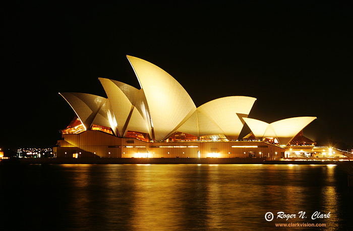
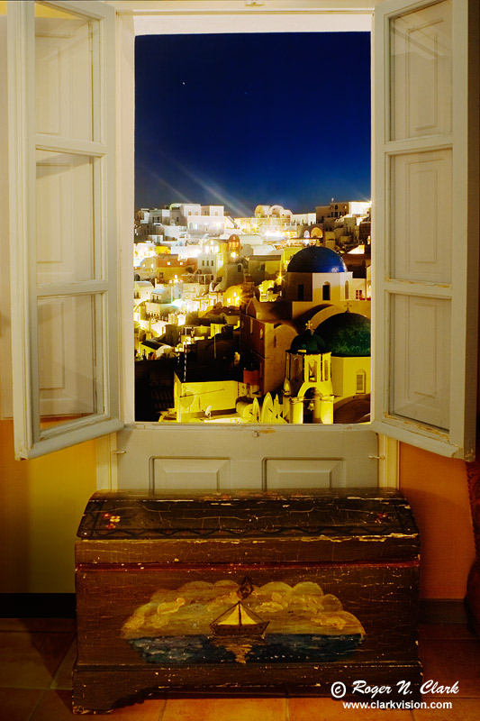
Night photography of cities with a DSLR is easily done with relatively short exposure times, as shown in Figure 2a. Use a low ISO setting to better fill the pixels resulting in better signal-to-noise ratios, an f/stop that gives enough depth of field and sharp images, and a few second exposure time. After each exposure, check the image and its histogram to see if more exposure is warranted. I usually do a wide range of exposures, like in the situation in Figure 2a where I did images from 1 second to 60 seconds. That way I could use a short exposure to maintain detail in the brightest portion of an image, and the longest exposure gets the faint detail. Multiple images could be combined if desired for recording a very high dynamic range. In this case, I found a single 20-second exposure to be ideal for the mood I wanted.
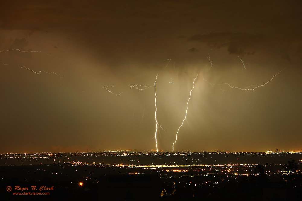
While lighting itself is not low light, recording it at night can be difficult (Figure 2b). One needs to keep the shutter open as long as possible to increase the chance of getting a strike. This image is the result of 3 minutes of exposure.
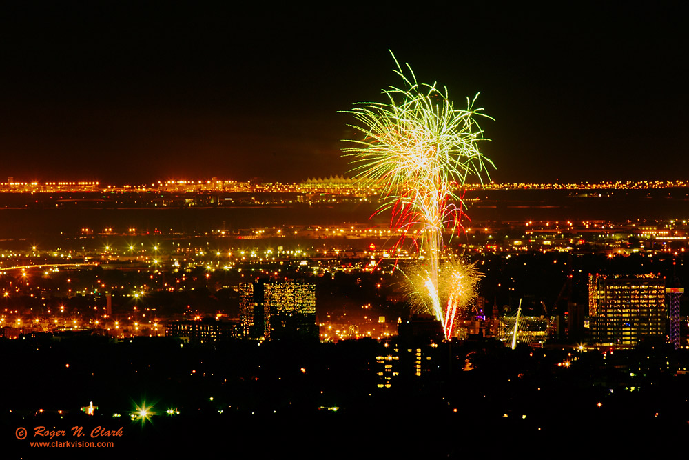
Lightning at night (Figure 2b) and Fireworks (Figure 2c) are momentary bright light sources in a darker environment. Exposure times must be long enough to include some interesting detail, so one must experiment with what balance of ISO, exposure time and f/ratio produces the best results. This will vary depending on how far away the light sources are. I usually start with ISO 100 and f/8 and adjust from there.
Indoor plus outdoor scenes are usually difficult to image because there is usually a large intensity difference. When people see my image displayed in Figure 2d, they often think it is a combination of two images pasted together. For this image, I balanced the number on indoor lights and waited for the twilight to reach just the right level and for the city light to come on. There was only a few minutes where the three light sources came to similar levels. When the light came together, a single exposure was all that was needed.
Low Light with Moving Subjects
The above low light photography was unconstrained by exposure time. One could in principle expose as long as one needed to record the image. But sometimes the subjects are moving and that necessitates exposures times shorter than might be desired to obtain a high signal-to-noise ratio.
Photographing a Moon rise (or set) can be difficult because of dynamic range. The Moon often appears much brighter than local surroundings, especially at night. Including city lights can add interest to the scene. But the rising Moon is moving, so the exposure can not be too long (Figure 3a). This necessitates an increase in ISO to shorten the exposure time. The example in Figure 2b had the moon rising through thick haze, which dimmed the light some, reducing the scene dynamic range while adding interest.
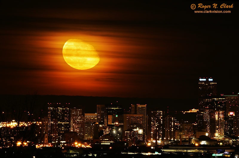
Note that the Moon high in a night sky is actually not a low-light target. The Moon is illuminated by the sun, so has near the same brightness as daytime terrestrial scenes. The Moon has about a stop lower reflectance than the typical Earth scene, so exposures are about a stop slower.
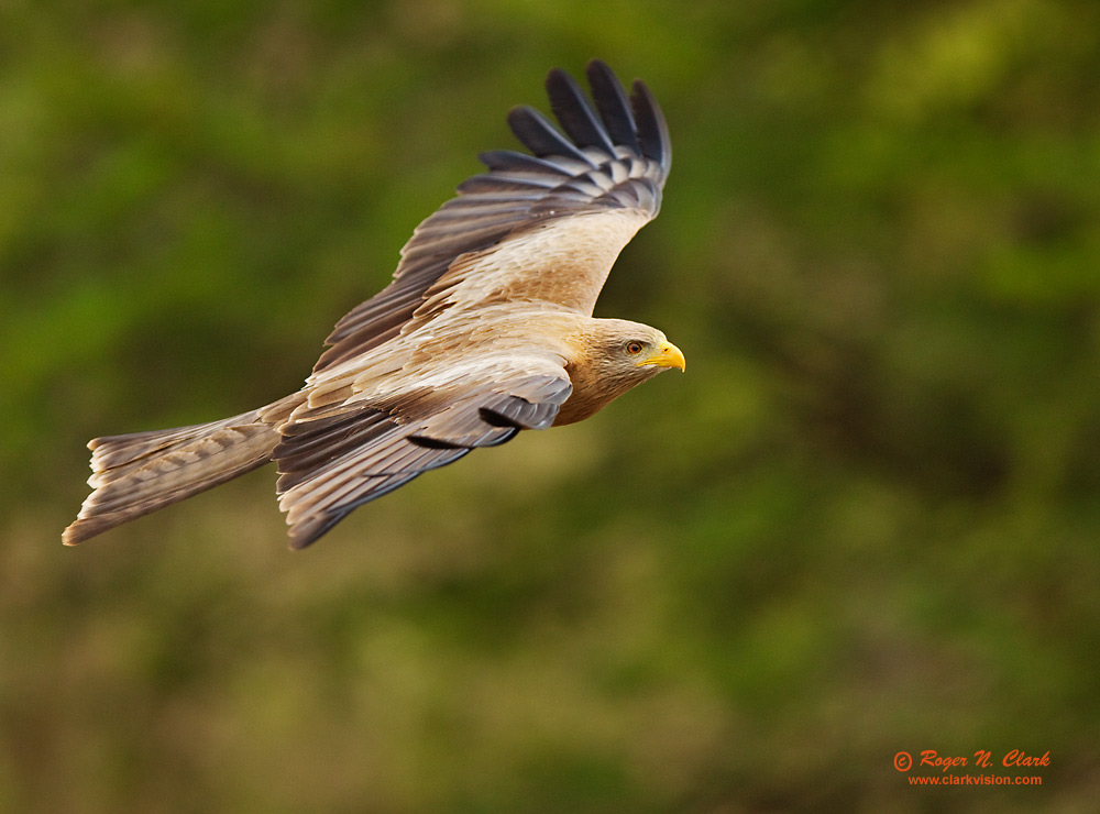
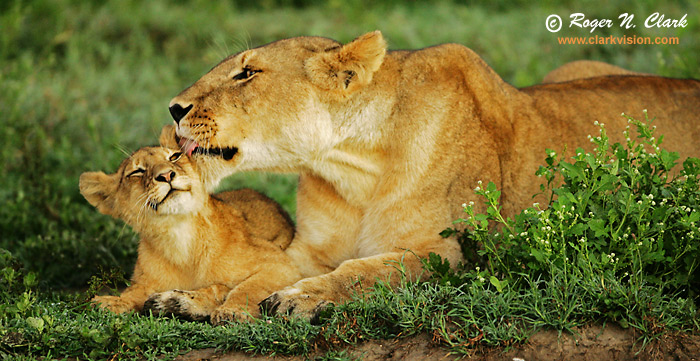
People and animals in low light are constantly moving and exposure times must be kept short enough to freeze any movement that one desires to be frozen. Examples are shown in Figures 3b and 3c. Because birds fly fast, a fast exposure time is necessary. I needed ISO 800 and a fast aperture of f/3.2 to freeze the action in overcast skies for the bird in Figure 3b, and even this fast of a shutter speed did not freeze the wing tips. For the mother lion and her cub in Figure 3c, I chose ISO 800 to give an exposure time of 1/80 second. I was lucky that movement was not too fast or I would have needed a higher ISO and shorter exposure time. It is better to have a noisy image than a blurred image in cases like this one.
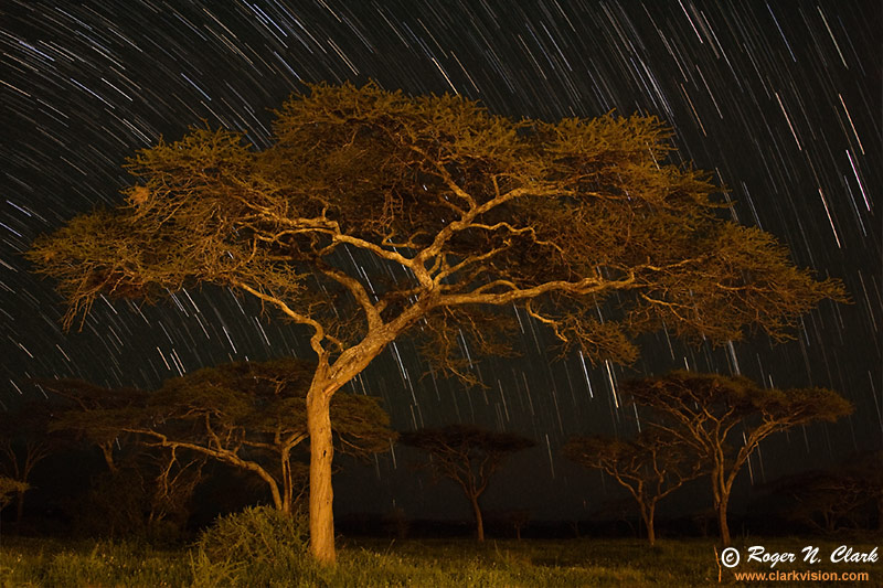
Sometimes movement can be good. Star trails are one such example (Figure 3d). But star trails by themselves may lack interest and including foreground subjects may add that interest. Figure 3d shows an example with acacia trees on the Serengeti lit by incandescent lights and star trails in the background.
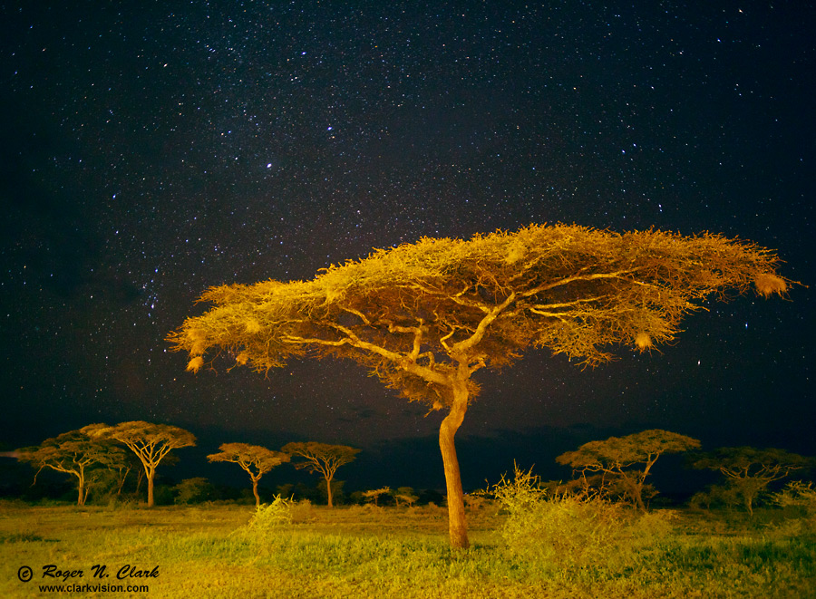
But sometimes we want to record stars and a local terrestrial scene with no movement of the stars or local scene. With a 35 mm sized sensor, and a 20 mm focal length lens, exposure times must be kept shorter than about 30 seconds or the rotation of the Earth will cause the stars to trail significantly. At 50 mm focal length, exposure times must be shorter than about 12 seconds. Figure 3e shows an example of a short exposure time (30 seconds) to prevent star trailing. The ISO was boosted to 3200 to increase the signal to record faint stars quickly (actually to amplify the signals from the faint stars above the electronics noise downstream of the sensor). The image in Figure 3e is in the same area as that in Figure 3d, but the images were taken about 4 years apart.
Long Exposure Deep Sky Low Light Imaging
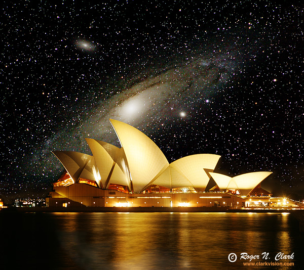
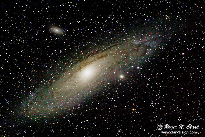
If one can track a moving subject, exposure times can be longer, even with low light. Imaging astronomical subjects is the ultimate in low light tracking. Figure 4a is one such example, the Andromeda galaxy. To make such images, a tracking mount was used that compensated for the rotation of the Earth.
Very Low Light Imaging
In order to show the effects and methods in very low light imaging, which might be scenes away from city lights with the light of the moon, or simply stars, or dark overcast nights, and astronomical imaging of faint stars, galaxies and nebulae, we need a controlled environment. A controlled environment was set up in a darkroom where experiments were conducted over several days. These tests illustrate how faint a signal can be recorded with a DSLR. The DSLR used was a Canon 1D Mark II. The performance of the camera used in the test is documented in Reference (1). In general, the best low light performance for this camera was found to be at ISO 1600 where the read noise is only 3.9 electrons and the gain is 0.81 electrons/camera 12-bit DN. Every electron generated is the result of the capture of one photon. With this calibration, the number of photons detected at each pixel in any image can be directly measured and the noise modeled. This allows us to explore the optimum for low light imaging methods with cameras like the 1D Mark II.
Some of the issues with very low light imaging is noise from dark current over long exposures. So one strategy developed by amateur astronomers using DSLRs for astrophotography is to do many shorter exposures. But every exposure suffers from read noise. Read noise is a constant amount of noise added to every image. You would like your signal to be large compared to the read noise, so read noise doesn't impact image quality.
Noise in an image is:
N = (S + r2 + t2)1/2 = (S + r2 + dc * e)1/2, (eqn 1a)
S = P * e, (eqn 1b)
Signal-to-Noise Ratio, SNR = S / N, (eqn 1c)
where N = total noise in electrons, S = number of photons (signal), r = apparent read noise in electrons (sensor read noise + downstream electronics noise), and t = thermal noise in electrons. The thermal noise equals the square root of the dark current per second, dc, times the exposire time in seconds, e. The signal, S, is proportional to the photon arrival rate, P, times the exposure time, e. Noise from a stream of photons, the light we all see and image with our cameras, is the square root of the number of photons, so that is why the S in equation 1 is not squared (sqrt(S)2 = S). Both the total photons counted, S, and the thermal noise, t, are functions of exposure time. S is directly proportional to exposure time. Thermal noise is is related to dark current. Dark current is usually expressed as electrons/second, and the noise is the square root of the electrons, so t is proportional to the square root of the exposure time.
A low light experiment was set up in a darkroom. A long exposure tests up to 30 minutes detected no residual light in the room. A white LED was covered with aluminum foil containing a pin hole, and a piece of white paper diffused the light. The light was pointed toward the direction of the target and using the known reflectances of squares on the target, equation 2 (below) was used to measure the light intensity illuminating the target. The light was measured at 0.00016 lux through the green filter of the Bayer filter. The full image of the test target is shown in Figure 5a, and the strip used for measurements and comparisons is shown in Figure 5b. The measured light recorded by the camera is shown in Table 1 along with a noise model using equation 1. The read noise for the camera is 3.9 electrons, and the dark current is 0.25 electrons/second at the temperature of the test (room temperature. 68 degrees F). For how these values were determined, see Reference 1 ( Procedures for Evaluating Digital Camera Noise and Full Well Capacities; Canon 1D Mark II Analysis http://clarkvision.com/articles/evaluation-1d2/index.html).
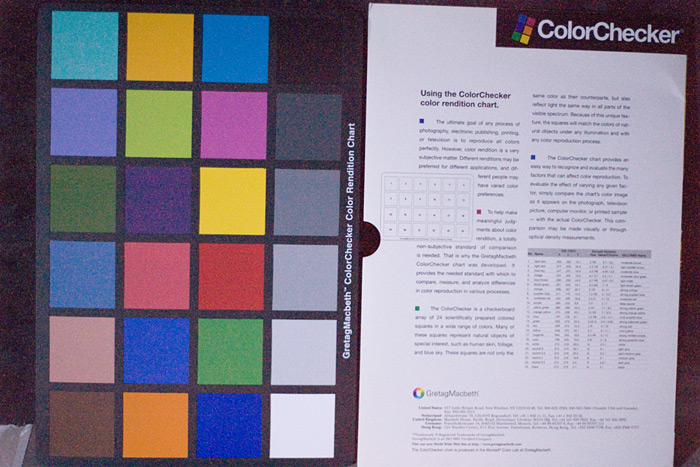
Figure 5a. The full image view of the test target for the 0.00016 lux light test.
This is a 632 second exposure at ISO 1600 with a Canon 1D Mark II with a 50mm
lens at f/1.8.
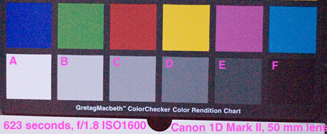
Figure 5b. A 623 second exposure of a target illuminated by only
0.00016 lux. The 1D Mark II camera was operating at room temperature
and ISO 1600 with a 50mm f/1.8 lens. This image has had no stretching
or processing other than raw image conversion in Photoshop
with default settings, then the two rows cropped
from the full image and down sampled about 4x.
The width of the image is the full height of the original image.
| Color Chart Patch |
Average Intensity (Photons) | Photon Rate (Photons per pixel/second) | Measured Noise (electrons) | Noise Model (electrons) |
| A | 749.4 | 1.21 | 26.9 | 30.3 |
| B | 494.9 | 0.794 | 24.0 | 25.8 |
| C | 288.7 | 0.463 | 22.7 | 21.4 |
| D | 148.5 | 0.238 | 21.4 | 17.9 |
| E | 60.6 | 0.097 | 21.2 | 15.2 |
| F | 19.4 | 0.031 | 16.8 | 13.8 |
Now let's examine working at lower levels by shortening the exposure time. There are three methods in use in the astrophotography community: 1) sum many short exposures to give a total long exposure time, 2) a few longer exposures summed together to give a total long exposure time, versus 3) single long exposures. An example of the difference between the two methods is shown in Figure 6 and Table 2. When working at low light levels, an important step is dark subtraction. Dark subtraction examples are shown later in Figure 7. At low levels digital cameras typically have a non uniform zero level as well as different offsets from pixel to pixel. But by taking a few images with the lens cap on, one can record what these offsets are, and use the dark images to subtract off the offset. This was done in the images in Figures 6 and 7.
Figure 6 shows a 623 second exposure of the test target sub-section with the gray patches studied labeled A, B, C, D, E, and F. Each test is called a set. Sets 1 and 2 are single exposures, while set 3 is six 10-second exposures combined with ImagesPlus 2.5 using sigma clipped median. Median combine reduces noise spikes due to hot pixels or spikes due to cosmic rays and other effects. A simple average of the images produces nearly the same result in this case. Note how the noise in set 3 appears similar to that in set 2. Square E is faintly seen showing that the camera is showing image detail while detecting less than 6 photons per pixel! The more interesting fact is, shown in set 3, that each exposure was detecting on average only 0.97 photons per pixel for patch E. With a read noise of 3.9 electrons, 0.97 electrons is only 25% of the noise. The reason we can see patch E is because the eye is integrating many pixels, averaging the noise. To first order, Figure 6 set 2 appears close to set 3, but set 3 shows fewer large noise spikes. The multiple exposures, when combined with dark frame subtraction, eliminates large noise spikes.
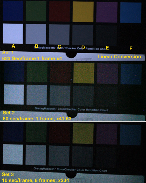 Figure 6. The test target from Figure 5. Set 1 is the same image from Figure 5b, but with a linear conversion. Each image is multiplied by the factor indicated. For example, you can recover the 16-bit tif file numbers by converting the image to 16-bit and dividing set 1 by 4, set 2 by 41.52, and set 3 by 234. The multipliers applied to each image is effectively an increase in ISO, or "digital ISO." Set 1 has an equivalent ISO of 3200, set 2 = ISO 66,450, and Set 3 = ISO 374,000! |
|
Now let's push a little fainter. Figure 7 shows Sets 2 and 3 from Figure 6 for reference. Set 4 shortens the exposure time to 1 second, showing 60 exposures combined using ImagesPlus 2.5 sigma clipped median combine, with dark subtraction (after the combine), and Set 5 shows just one of those 60 exposures, also with dark subtraction. Note the number of photons detected on each patch. In Set 4, patch E is faintly visible but not as well as it is in Set 3. Even though the total exposure time is the same, the read noise from each exposure in Set 4 contributes to the noise in the final image. The fact that patch E is faintly visible in Set 4 shows that the camera can record only 0.1 photon per pixel per image and if enough images are added, image detail can be recorded. Obviously, as the photon count rises, the image quality improves. Patch D in Set 4 appears distinct even though only 0.24 photons per pixel per frame are recorded. Patches C and B show more cleanly despite recording only 0.46 and 0.79 photons per pixel per frame. All patches in Set 4 have noise 3 to over 100 times fainter than the read noise of 3.9 electrons per pixel per frame. While 0.1 photons per pixel per results in detectable image detail, totaling about 6 photons, patch D, at 0.03 photons per pixel per frame, totaling only 1.9 photons, does not show a detection. A reasonable conclusion is that the total signal after combining multiple images should be greater than the read noise for one frame.
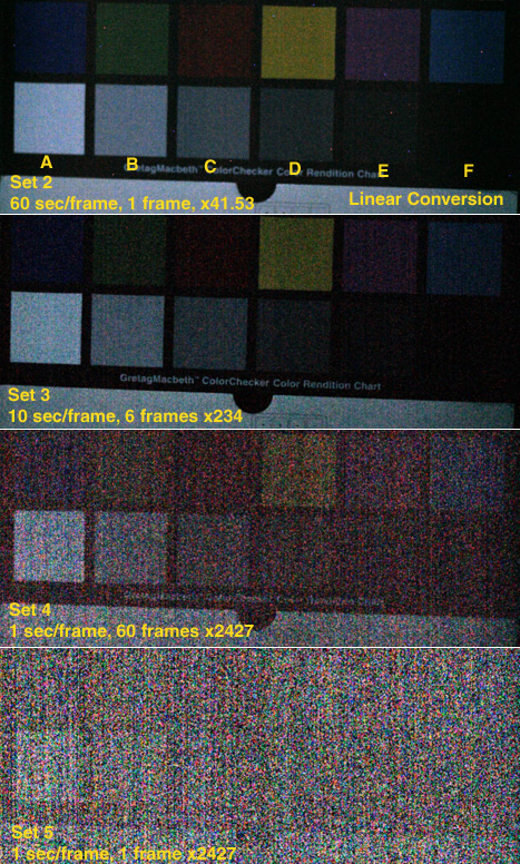 Figure 7. The equivalent ISO's for the single frame images are: Set 2 = ISO 66,450, and Set 5 = 3,883,000. |
Light Intensities Under Different Lighting Conditions So what are typical light levels one might encounter in real-world conditions? Table 4 shows the relative brightness scale and common subjects (derived from Reference 5). Several units are used in the table, the stellar magnitude equivalent of the illuminating source, the Luminance at the Earth's surface, and what the camera exposure would be to properly expose an 18% gray card. The brightnesses of astronomical objects is measured in stellar magnitudes, with the star Alpha Lyra forming a reference = 0 at all wavelengths. It is an absolute scale whose units are the brightness of the star Alpha Lyra. The Stellar Magnitude is a log scale with one magnitude equal to the fifth root of 100, or 2.51188643, and larger numbers mean fainter. Table 4
                                    Stellar    Luminance at     Camera
                                   Magnitude  Earth's surface   Exposure
                                            (lumens/sq. meter)  Time on 18%
                                                  (lux)         gray card
Sun overhead                          -26.7    130000          1/600s f/8 ISO100
Full daylight (not direct sun)    -24 to -25    10000-25000
Overcast day                          -21        1000           1/4s  f/8 ISO100
Very dark overcast day                -19         100           1/4s  f/4 ISO200
Twilight                              -16          10             1s  f/4 ISO400
Deep twilight                         -14           1             3s  f/2 ISO400
1 Candela at 1 meter distance         -13.9         1.00          3s  f/2 ISO400
Full Moon overhead                    -12.5         0.267         3s  f/2 ISO1600
First or Last Quarter Moon, overhead  -10.0         0.027        30s  f/2 ISO1600
Total starlight + airglow              -6           0.001       775s  f/2 ISO1600
Venus at brightest                     -4.3         0.000139
Total starlight at overcast night      -4           0.0001      970s  f/1 ISO3200
Sirius                                 -1.4         0.0000098
0th-mag star                            0           0.00000265
1st-mag star                           +1           0.00000105
6th-mag star                           +6           0.0000000105
A camera's light meter can be used to measure lux. The formula is
comes from the definition of ISO (see Reference 2, and references therein)
lux = 12.4 * pi * f/#2 / (R * t * exposure_time * ISO), (eqn 2) where f/# is the f/number of the camera lens, exposure time is in seconds, ISO is the ISO speed, R = reflectance of the target, t = lens transmission, and pi = 3.14159. Equation 2 can be simplified with some assumptions. If we assume white paper with 90% reflectance (use a stack of several sheets), R = 0.9, and assume the optical transmission, T = 0.7, then Equation 2 reduces to: lux = 62 * f/#2 / (exposure_time * ISO), (eqn 3) For example, I measured the exposure time on white paper in full sunlight at 1/3000 second at f/8, ISO 100. Equation 3 gives the lux from the sun as 119,000, agreeing within 10% of the value in the above Table 4. If you want to use an 18% gray card, the factor 62 becomes about 310. A Moonlit Scene As a test of a low light situation and what can be recorded in a real scene, a country road outside of a city with distant mountains was imaged when it was illuminated by the moon 1 day after first quarter. Assume we may want to image fast to record moving objects, like an animal, person, or license plate of a passing car. If not for the movement, we could simply expose for a longer duration and obtain a beautiful image. The predicted illumination of our moonlit scene was 0.06 lux. Assuming an average reflectance of 18%, and finding an exposure of 10 seconds produced a well-exposed scene, equation 2 gives 0.06 lux, in agreement with prediction. By reducing exposure time, we can observe how image quality is reduced due to fewer photons and the camera's read noise. Images were recorded in raw and jpeg mode. with exposures range from 10 seconds to 1/20th second on a Canon 1D Mark II camera at ISO 1600, using a 50mm f/1.8 lens. Raw data were converted with a linear conversion using ImagesPlus 2.5. A second raw conversion was also done with the same software and a standard transfer curve. The linear data were used to determine the number of photons detected. At ISO 1600, the gain is 0.81 electrons/12-bit camera DN, and the maximum number of photons (4095 camera DN) is (4095*0.81=) 3317. The read noise at ISO 1600 is 3.9 electrons (Reference 1)
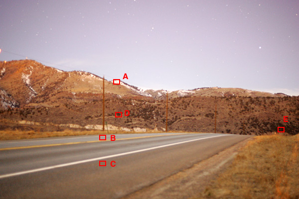 Figure 8. The moonlit test scene: a 10 second exposure at ISO 1600, f/1.8. Patches A-E photon statistics are shown in Table 5. The number of photons detected in patches A-E is given in Table 5. Figure 9 is the same as Figure 8, without the text and boxes to show the highest signal-to-noise ratio image detail. Figure 10, a 1-second exposure shows that a decent image can be acquired with only a few tens of photons. Less than about 10 photons per pixel still forms a color image where significant detail can be recognized. But at this level, non-uniformities in the dark level become a limitation (Figures 12, 13). For such low levels, a dark frame subtraction can push limits even lower (Figure 14). In Figure 14, where photon counts are similar to and less than 1 photon per pixel per frame, image detail is still visible but only with significant noise. Note the average signal-to-noise ratio per pixel is about 0.25. Finally, combining a few of these short exposures again provides a better image (Figure 15).
Table 5
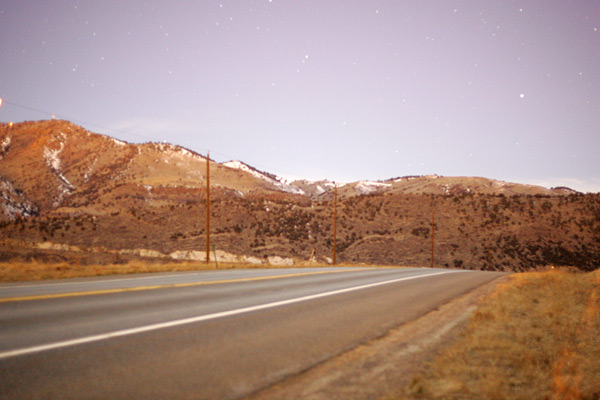 Figure 9. The moonlit test scene: a 10 second exposure at ISO 1600, 50mm, f/1.8, no dark subtraction. Same image as in Figure 8. The number of photons recorded in Patch B, mid-level gray, was only 382 per pixel.
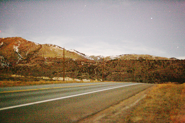 Figure 10. The moonlit test scene: a 1 second exposure at ISO 1600, 50mm, f/1.8, no dark subtraction. The image was stretched to give a similar histogram distribution as the 10-second exposure. The number of photons recorded in Patch B, mid-level gray, was only 38.2 per pixel. Note: this is the image quality one would expect if the ISO of the camera were set at 16,000! Even though the camera has no such setting, one can achieve it by digital post processing.
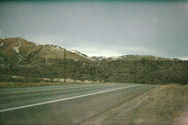 Figure 11. The moonlit test scene: a 0.25 second exposure at ISO 1600, 50mm, f/1.8, no dark subtraction. The image was stretched to give a similar histogram distribution as the 10-second exposure. Patch B, mid-level gray, recorded only 9.5 photons per pixel. Note the bright patch in the lower right corner. This is due to non-uniform and non-zero black level. This non zero black level is measured by taking a dark frame (see Figure 12). This image has an equivalent ISO = 64,000.
 Figure 12. Dark frame obtained with a 0.05 (1/20) second exposure and the image multiplied by 512. Linear conversion to a 16-bit tif file with ImagesPlus 2.5. This image is an ImagesPlus sigma clipped median combine of 64 dark frames. The median combine reduces noise spikes, but is similar to an average. The bright spots in the lower right corner and along the bottom edge are due to heating from camera electronics. All digital cameras will have these effects, but not necessarily this exact pattern.
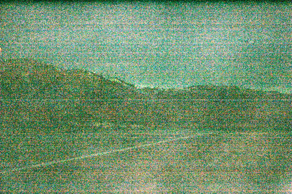 Figure 13. The moonlit test scene: a 0.05 second exposure at ISO 1600, 50mm, f/1.8, with no dark subtraction. The image was stretched to give a similar histogram distribution as the 10-second exposure. Note the dark frame pattern from Figure 12. This image has an equivalent ISO = 320,000.
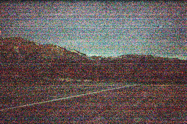 Figure 14. The moonlit test scene: a 0.05 second exposure at ISO 1600, 50mm, f/1.8, with dark subtraction. The image was stretched to give a similar histogram distribution as the 10-second exposure. This is Figure 13 minus Figure 12 (using linear data then stretched). The dark subtraction reduced the pattern noise. The bright snow patches received only about 7 photons per pixel. Patch B, mid-level gray, recorded only 1.9 photons per pixel and darker portions of the image recorded less than 1 photon per pixel. With read noise of 3.9 electrons per pixel, most of the image has a photon signal less than the read noise. This image has an equivalent ISO = 320,000. To see the image at full size, click here (NOTE: it is 11.5 megabytes and S/N < 1 appears very noisy; you will need to print it to view the information because on screen the pixels are too large for the eye+brain to effectively integrate. This image was stretched independently from Figure 14, as that stretch was not saved at the original full size). The image data were multiplied by 512 for viewing, so the maximum signal in the original (dark subtracted) file was less than 128 out of 65535. What you will see if you print the image is about the same detail as seen in the Figure 14 image, perhaps a little more as your eye integrates pixels to extract image information.
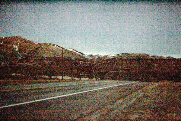 Figure 15. The moonlit test scene: 64 frames, each 0.05 second exposure at ISO 1600, 50mm, f/1.8, with dark subtraction were combined with ImagesPlus 2.5 using sigma clipped median combine. The final image was stretched to give a similar histogram distribution as the 10-second exposure. This images proves that when multiple images are combined, less than one photon per pixel per frame can be accumulated to show significant image detail. Compare the noise in Figures 10 and 15. Figure 10, with an exposure time of 1 second in one exposure, has less noise than the 3.2 second equivalent of the image in Figure 15. The noise model (equation 1) shows Patch B of Figure 10 has a signal-to-noise ratio of (38.2/sqrt[38.2 + 3.92 + 0.25] =) 5.2 and in Figure 15 of (sqrt(64)*1.9/sqrt(1.9+ 3.92 + 0.05] =) 3.7. Thus, the visible noise in the two images is what we should expect. This illustrates that while you can dig signal out of the noise with multiple exposures, longer exposures can produce better results. If the sensor had no read noise and no thermal noise, the images would be photon noise limited and Figure 10 would have a signal-to-noise ratio of 6.2 and Figure 11 would have 11. For images with a few tens of photons per exposure, signal is sufficient that read noise becomes insignificant and the sensor is essentially photon noise limited. This means that to improve the signal to noise further in this imaging situation would require a sensor with higher quantum efficiency. The Canon 1D Mark II sensor quantum efficiency is about 38% (Reference 2), so improvements of up to almost 2.6 are possible, and a little more with improvements in optics transmission. Another way to deliver more light is to use a faster f/ratio lens. Comparing results from the moonlight scene and the much lower light level darkroom test shows an interesting difference in the photons per pixel. The higher light level moonlit scene requires higher photons/pixel per frame to see image detail. This is because of the complexity of the moonlit scene, and has nothing to do with light levels. In such complex, real world scenes, practical limits are a half to 1/3 of a photon per pixel per frame. Astronomical Imaging The ultimate in low signal detection is imaging faint stars, galaxies, and nebulae. Reference 2 shows that the signal received from the reference star Alpha Lyra by the Canon 1D Mark II camera through the green passband and a 500 mm f/4 lens is about 1,1950,000 photons/second through the Earth's atmosphere (with average extinction). From that, we can compute how many photons fainter stars would record (Table 6). The photons/minute = 60*A/(10^(0.4*M)), where A = the 1,1950,000 photons/second from Alpha Lyra with that 5-inch aperture lens, and M is stellar magnitude. Table 6
Recording surface brightness is another issue for detecting light from galaxies and nebulae. The 5-inch aperture (125 mm) 500 mm lens on a 1D mark II camera gives 3.38 arc-seconds/pixel with 8.2 micron pixel spacing (= 3600 *arc tangent(0.0082/500 ~ (0.0082/500)/206265). Adding a 1.4x TC reduces that to 2.42 arc-seconds/pixel. The angular area is 11.4 square arc-seconds per pixel at 500mm and 5.86 square arc-seconds per pixel at 700mm (500 mm with the 1.4x TC). Now we can compute the photons the camera plus lens would record for different surface brightnesses (Table 7). Table 7
Note: Photons/minute are converted photons in the sensor, not photons incident on the sensor. Discussion Using the photons/minute in Table 7, you can compare the expected total photons in an astronomical image to the results in Figure 8 to 15 to see what kind of signal and noise you might expect when imaging astronomical objects. Faint parts of galaxies are in the surface brightness 24 and 25 magnitudes per square arc-second range and fainter. Galaxies tend to have surface brightnesses in the 17 magnitudes per square arc-second in their cores with fainter outer parts, while nebulae such as that in the Pleiades (M45) runs about 20 magnitudes per square arc-second and fainter (see References 3, 4). The bright core of the Orion Nebula, the Trapezium, in M42 has surface brightnesses in the 16 to 17 magnitudes per square arc-second range. Images that reach to 21 to 22 magnitudes per square arc-second show the beauty of many galaxies and nebulae, but the signal may appear a little noisy at the low end. Longer exposures reaching 24 magnitudes per square arc-second will appear smoother, but can require hours of exposure. Improving Photon Collection With existing technology, basic physics tells us how to record more light. 1) Faster lens. 2) Bigger sensor with correspondingly larger lens. 3) Larger pixels in a trade of spatial resolution for collecting more light per pixel with a given lens. 1) Faster lens. A faster lens (lower f/ratio), collects more light and delivers more light per square micron into the sensor. For example, an f/2 lens will deliver 4 times the light of an f/4 lens. 2) Bigger sensor with correspondingly larger lens. The larger lens, even at the same f/ratio, collects more light, thus delivering more light per angular area than a smaller lens of the same f/ratio. Given two sensors, one twice as large are the other, and with a lens twice the focal length, but the same f/ratio on both cameras, the 2x bigger lens delivers 4 times the light for the same field of view. This is the basic reason why small sensor P&S cameras have poor low light performance compared to larger sensor DSLRs. For more on this topic, see: Does Pixel Size Matter? 3) Larger pixels in a trade of spatial resolution for collecting more light per pixel with a given lens. A lens of a given f/ratio delivers X photons per square micron. If the pixel is larger, it obviously covers more square microns, so collects more light. But the larger pixel spacing records less detail. This is the basic design philosophy behind cameras like the Nikon D3 and Canon 1D Mark II, which both have pixels over 8-microns in size (so over 64 square microns in area). An example of such a trade is shown in Figure 16. For more on this topic, see: Telephoto Reach and Digital Cameras.
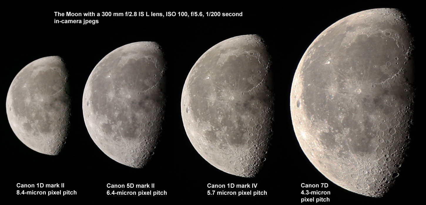 Figure 16. The Moon photographed with 4 different cameras using the same lens, so focal length is the same for each image. This is the full resolution image produced in the camera and written as a jpeg file. No post processing sharpening has been done. Cameras like the 1D Mark II and Nokin D3 will produce images like that on the left. The signal-to-noise ratio per pixel is highest for these cameras. Cameras with smaller pixels will show more detail (moving to the right), but signal-to-noise ratio per pixel drops. Which image do you prefer: the high signal-to-noise ratio pixels in the images on the left versus the lower signal-to-noise ratio pixels in the images on the right? Comparing results in Figure 16, I had plenty of light, so each image has a good signal-to-noise ratio. As light levels drop, the images from cameras with smaller pixels will show more noise per pixel. Thus, depending on ones tolerance for noise, different cameras will produce better results under varying situations. Each camera with different pixel and sensor sizes is like a different tool that work best in different situations. Future Technology There are several ways for the camera to detect more photons for future technology. 1) Improve the transmission of the optical system. If the optics had 100% transmission, the improvement would be less than a factor of 2. 2) Improve quantum efficiency. I measured the 1D Mark II's QE as 28% (Reference 2), so about a 3.6x improvement is possible. Back-side illuminated CCDs have QEs in the 90+ % range, so ~3x is feasible. 3) Monochrome Sensor. If you do not need color, the Bayer filter could be removed. The bandpass of the green filter, for example, is about 0.077 microns, and the spectral width of the sensor is about 0.7 microns, so a factor of about 9 for bandwidth and at least another 10% for transmission would result in a 10X improvement. The raw sensor ISO would then be on the order of 16,000 instead of 1600! But the large wavelength range would require new lenses as most lenses are not color corrected from the UV to the infrared where the sensor responds. It would also give unusual black and white response (more like black and white infrared film). There are applications were such full wavelength range imaging is done, as in low light night vision video applications. But for color imaging, the low noise DSLRs are working amazingly well and the tests here show low noise DSLR sensors could compete in some of those situations. Other Digital Cameras The examples on this page used only a few high-end model digital cameras. But the low light performance of these cameras are similar to other digital cameras as shown in Reference 6 ( Digital Camera Sensor Performance Summary). The astrophotograph of the Pleiades (M45) in Reference 4 ( Surface Brightness of Nebulae in M45) was taken with a Canon 10D digital camera. As technology moves ahead, there is better control of fixed pattern noise, so newer technology cameras generally perform better. A demonstration of pixel and sensor size in night photography is illustrated in Reference 9 ( Digital Cameras: Does Pixel Size Matter? Part 2: Example Images using Different Pixel Sizes) which shows increased noise (due to fewer photons being collected) with the camera with small pixels and a small sesnor. For small sensor cameras with small pixels, one would need to take many short exposures (a few seconds each) and add the images together. To see the performance of digital cameras to the faintest light, see Figures 6 and 7 in Reference 6 ( Digital Camera Sensor Performance Summary). Because the electronic sensors in digital cameras have high quantum efficiency compared to film, and because electronic sensors do not suffer from reciprocity failure as does film, large pixel digital cameras can detect lower light levels in shorter time than film. Conclusions Digital Cameras are capable of detecting small numbers of photons and making credible detections of image detail. If multiple images are added together, or multiple pixels are added, photon rates of less than 1 photon per pixel per frame can still result in detectable image detail. However, for beautiful smooth images, hundreds of photons are required. Low light imaging is a compromise in recording enough light in the time one needs to limit blur. Static scene that can be exposed for a long time (e.g. with a tripod) cam be imaged with with enough exposure to obtain relatively low noise images. Moving subjects in low light require fast lenses and large sensors to capture enough light to obtain acceptable signal-to-noise ratios.
References 4) Surface Brightness of Nebulae in M45 http://clarkvision.com/astro/surface-brightness-profiles/m45. 5) Clark, R.N., Visual Astronomy of the Deep Sky, Cambridge University Press and Sky Publishing, (book of 355 pages), 1990. 6) Digital Camera Sensor Performance Summary http://clarkvision.com/articles/digital.sensor.performance.summary 7) The f/ratio Myth and Digital Cameras http://clarkvision.com/articles/f-ratio_myth 8) Digital Cameras: Does Pixel Size Matter? http://clarkvision.com/articles/does.pixel.size.matter 9) Digital Cameras: Does Pixel Size Matter? Part 2: Example Images using Different Pixel Sizes http://clarkvision.com/articles/does.pixel.size.matter2 10) A 20 minute total exposure time comparison between film and digital: http://www.aoc.nrao.edu/~whwang/misc/D200_vs_film
The Night Photography Series:
http://clarkvision.com/articles/night.and.low.light.photography
First Published February 24, 2006 | ||||||||||||||||||||||||||||||||||||||||||||||||||||||||||||||||||||||||||||||||||||||||||||||||||||||||||||||||||||||||||||||||||||||||||||||||||||||||||||||||||||||||||||||||||||||||||||||||||||||||||||||||||||||||||||||||||||||||||||||||||||||||||||||||||||||||||||||||||||||||||||||||||||||||||||||||||||||||||||||||||||||||||||||